Master's thesis of Applied Science: An investigation into the identification of objective parameters correlating with the subjective functional performance of critical listening rooms

An Investigation into the Identification of Objective Parameters Correlating with the Subjective Functional Performance of Critical Listening Rooms

A thesis submitted in fulfillment of the requirements for the degree of Master of Applied Science

J. L. Watson B.App. Sci. (App. Phys.)

School of Applied Sciences Science, Engineering and Technology Portfolio RMIT University March 2006

Declaration:

I certify that except where due acknowledgement has been made, the work is that of the author alone; the work has not been submitted previously, in whole or in part, to qualify for any other academic award; the content of the thesis is the result of work which has been carried out since the official commencement date of the approved research program; and, any editorial work, paid or unpaid, carried out by a third party is acknowledged. March 20, 2006

Acknowledgements: Firstly, I would like to thank all of the staff of the School of Applied Physics at

RMIT for the employment, the flexibility and help in performing the work required for

this research.

Extra special thanks is extended to my two main supervisors, Associate Professor

John Davy and Doctor Elizabeth Lindqvist for offering me the opportunity to pursue this

research and then providing multitudes of encouragement despite the sometimes

melancholy attitude of my student self. Thanks also to my second supervisor, Doctor Neil

McLachlan, for providing valuable insights into perceptual aspects of sound and for

sharing a similar enthusiasm for the sensation of sound.

Superlative thanks to my friend, employment supervisor and scientific mentor

Peter Dale. I especially appreciate his unwavering support of my research to his own

occasional inconvenience but especially appreciate his calming and helpful nature.

I would also like to extend thanks to the multitudes of people who participated in

the research. Special thanks are justified to the owners of the surveyed critical listening

rooms and the professional listening subjects. Thanks so much for the access to your

facilities and all of the illuminating informal chats as part of arranging access to such

facilities.

Thanks also to my friend Ben Butler for his very helpful feedback in the later

parts of the writing process. Consequently, it became obvious, particularly after

consultation with my supervisors, that I was prone to repetition in my writing style and

also likely to write a sentence that is probably way too long resulting in meandering

sentence structure and mentioning the same things repeatedly.

Also deserving of thanks are my mother Pinky, sister Victoria and her husband

Robbo. I’d also like to thank the new arrival, my nephew William, and look forward to

his thoughts on the subject matter discussed in this thesis.

Finally, I’d like to dedicate this research to my late Father whose counsel, love

and encouragement I miss everyday.

iii

Table of Contents:

Reference Section Title:

Title Page Declaration Acknowledgements Table of Contents Summary 0.1 0.2 0.3 0.4 Page Number i ii iii iv 1

1 1.2 2 3

1.3 1.4 1.5 1.6 1.7 1.8 1.9 Background to the Research The Need for Consideration of Subjective and Objective Parameters in Critical Listening Room Acoustics Objective Measurements and Considerations Methods of Analysis of Objective Data Limitations of Objective and Subjective Measurement Psycho-acoustic and Perceptual Measurements Aims of the Research Content and Organisation of Thesis Chapters Summary 4 10 15 17 19 19 20

2 2.1 21 22

2.2 30

2.3 34

2.4 2.5 Evaluation of Objective Measurements Analysis and Comparison of Objective Acoustical Parameters as Measured by Different Methods 2.1a Laboratory Measurements – Reverberation Time Comparison: 2.1b Real Critical Listening Room Measurements – Reverberation Time Comparison Evaluations of the Salience of the Objective Measurement Methods Other Considerations for the Implementation of the chosen Objective Method in The Field Perceptual Aims and Considerations Summary 35 39

Table of Contents (continued): Reference Section Title:

Experimental Methodology in the Field Objective Methodology and Instrumentation Limitations Subjective Methodology in the Field Summary Page Number 40 40 49 49 3 3.2 3.3 3.4

51 52 54 4 4.1 4.2

56 71 79 85 88 88 89 4.3 4.4 4.5 4.6 4.7 4.8 4.9

91 97 4.10 4.11

Results and Discussion Impulse Response Notes Noted Non-Acoustical Characteristics of Critical Listening Rooms Measured Acoustical Parameters Case Study: Room 2 Case Study: Room 6 Other Statistical Analyses Limitations of Objective Analysis Outline of Subjective Investigations Summary of Objective Measurements of Room in which Subjective Research Performed Some Initial Results of Subjective Investigations Variations in Subjective Investigations to Attempt to Yield Useful Data General Evaluation of the Results 98 4.12

Summary and Conclusion Objective Measurement Summary Subjective Investigation Summary Further Work Summary 105 105 107 108 110 5 5.1 5.2 5.3 5.5

References 111 6

117 Appendix I Acoustical Parameter Results including Reverberation Times and Early Decay Times

Summary:

The link to subjective parameters and objective parameters in the field of room

acoustics has been the source of much research. This thesis surveys some of the available

objective room acoustical analysis methods, quantify their advantages and disadvantages

with respect to the measurement of acoustical qualities of professionally operated critical

listing rooms, and implements these methods in a range of critical listening rooms. In

conjunction with the objective room analysis, a subjective component of research was

also performed. A series of anechoically recorded standard instrument sounds were

presented to professional listeners in their critical listening spaces with the listeners asked

to alter the sounds to taste: to “mix” the sounds. Anechoic sounds were used as they had

no room effects recorded as part of the original signal. The subject, as part of the

“mixing” process, was asked to add artificial reverberation and equalisation to their taste.

The original sounds were objectively compared to the “mixed” sounds. It was hoped that

this comparison would result in correlation between aspects of the objective critical

listening room analysis and the subject’s response to the anechoic signals when

superimposed with their critical listening room acoustics as part of the “mixing” process.

The research generated multitudes of data as the objective component of the

research was performed in 17 professionally operating critical listening rooms and

included 4 anechoic mixing sessions with 1 subject. The discussion presented in the body

of the thesis includes comparison between different room analysis methods implemented

both in the laboratory and in the field and also discussion of the results of the

implementation of the selected room acoustical measurement methods in the critical

listening rooms measured as part of the research. Statistical comparisons were performed

on different aspects of the data collected. Also discussed are the subjective responses to

the anechoic stimuli and the problems in attempting to objectively analyse such

complicated perceptual responses. The attempt to find an objectively measurable

parameter that correlates with subjective impression was unsuccessful. More specifically,

the research demonstrated the complicated relationship between the objective and

subjective in critical listening rooms.

Title of Thesis: An Investigation into the Identification of Objective

Parameters Correlating with the Subjective Functional Performance of Critical

Listening Rooms

1 Background to the Research

Designers in many different disciplines have long attempted to find objective

methods of accomplishing subjective goals. The field of sound is no different in this

respect. This research is an attempt to investigate measurable objective acoustical

parameters of a space and to attempt to establish links between these objective parameters

and repeatable analysis of the subjective functionality of the space.

A critical listener is a person who makes decisions professional, creative,

recreational or otherwise based on their subjective response to sound. Broadly speaking,

critical listeners would include audio engineers, musicians, music lovers and record

producers. The spaces in which these people make their aural decisions would hence

qualify as a critical listening room. It is the subject of this research to investigate

measurable objective parameters in these critical listening rooms. Then to attempt to

correlate the critical listeners’ subjective response to the room through these

measurements of objective parameters. To further narrow the scope of the research, it was

decided to objectively investigate recording studio control rooms and professional

listeners. This decision was taken to attempt to improve the repeatability of the subjective

aspects of the research through the use of professional listeners. In the objective domain,

with the broad assumption that recording studio control rooms have similar acoustical

traits, it was also anticipated that direct comparison of the objective qualities of the rooms

might be found to be possible. The surety with which these professional listeners and

audio engineers are able to make their decisions is of paramount importance to their

success as professionals. Such professional listeners also have trained themselves to be

able to ‘turn on’ their listening skills when required. Professional listeners will also be

particularly sensitive to the acoustical quality of the environment in which they are

making decisions. Consequently, listening rooms have been designed around their aural

requirements and demands. It is the object of this research to objectively attempt to

discover acoustical parameters that have a perceptual relevance in the context of a

professional listener in their own room.

The world of critical and professional listening is defined by a vast array of

parameters found in disciplines that are diverse and varied. If there exists a complicated

relationship between these diverse parameters that leads to a functional critical listening

room suitable for all critical listeners then it has eluded researchers to this date. To

examine the question of a decipherable link between objective and subjective parameters

in critical listening rooms, it is instructive to examine some of the characterizations of

these parameters. These parameters can be categorized as being exclusively or

collectively subjective or objective and range from the most technical to the most human

in origin. It is then obvious that these parameters can directly affect the perceived quality

and success of the output from critical listening sessions.

1.2 The Need for Consideration of Subjective and Objective Parameters in Critical

Listening Room Acoustics

There has been much research and testing performed on critical listening rooms

with varying amounts of objective emphasis being placed on the subjective evaluation of

the functionality of the critical listening room. Commonly, these subjective evaluation

tests are in the form of listening tests by those that will work and/or design the critical

listening room (Jordan, 1969; Davis, 1980; Walker, 1995) and to a lesser degree, by those

who will be consuming the output of the critical listening room (Jordan, 1969; Holman,

2000). Whilst subjective tests are a useful method of evaluation, they are both expensive

and time consuming to undertake, and they require the training of an expert listening

panel in order for them to give consistent and reliable results. Even then, each listener

will have their own distinct subjective impression of the acoustics of the room. Thus a

critical listening room iteratively designed and altered based on subjective listening tests

of a large number of critical listeners will never sound ‘good’ to all critical listeners. As

an alternative to subjective methods of evaluation, objective measures that correlate well

with certain subjective parameters would be more accurately repeatable, and could save

time and money (Grewin 1995). Therefore it would be useful if subjective assessments

could be replaced or complemented by objective measurement methods.

The quality of a critical listening room is a multidimensional prospect that is

dependent on the properties of a large number of subjective and objective parameters. In

view of this, in order to create an objective measurement that is related to the overall

quality, it is necessary to quantify the properties of each of the parameters that contribute

to the perceived quality of a sound. Therefore, in order to develop an objective

measurement of overall sound quality, it is necessary to initially consider single

parameters or small groups of parameters and attempt to create objective measurements

that relate to these.

1.3 Objective Measurements and Considerations A range of room acoustical analysis techniques were investigated as part of the

research. Loosely, the techniques investigated can be broken up into two distinct

categories: Impulse Response and Direct Measurement. Impulse response techniques

involve the measurement, either directly or indirectly, of the impulse response of the

critical listening room under test. Direct Measurement methods involve the measurement

of a particular acoustical quantity i.e. “Reverberation time” or “Clarity”. It is worth

noting that many acoustical parameters can be measured through both the direct method

and the impulse response method.

Since the research being undertaken was quite broad in scope, it was desirous to

minimize the amount of limiting decisions with respect to measurement and analysis. In

other words, the data was taken so as to be analyzable in the maximum number of

different ways as dictated by the research. For these reasons, and fairly early on in the

course of the research, the advantages of pseudo-random noise (maximum length sequences, inverse repeated sequences1) and swept sinusoidal methods of impulse

response measurement were realized: an impulse response contains information that can

be analyzed in a number of ways. Impulse response methods are also a very common

experimental technique and there are consequently well enunciated testing methods in

1 An inverse repeated sequence is simply two maximum length sequences placed back to back but the second sequence is inverted ie in the second sequence a 1 from the first sequence is changed to a 0 and vice versa. This slight alteration is incorporated into the deconvolution procedure.

many branches of physics. Additionally, if the duration of the pseudo-random noise was

roughly equal to the reverberation time, it was possible to do direct decay measurements

in conjunction with impulse response measurements by treating the pseudo-random noise as broadband noise2.

Many standard acoustical texts (Everest 2004, Kinsler 2000, Kuttruff 1991)

provide good outlines and references for competing room analysis methods. Whilst the

texts will often discuss the different methods and the similar measurements they perform,

they generally do not compare the differences in the technical precision or accuracy of

the different methods. Accordingly, upon commencing the research, a large range of

objective room analysis methods were researched and practically compared on the levels

mentioned above. The different methods investigated were:

Impulse Response Measurement: Maximum Length Sequence (MLS), Inverse Repeated

Sequence (IRS), Swept Sinusoid, Impulsive Sound Excitation (i.e. gunshot or balloon).

Direct Measurement: Time Delay Spectrometry (TDS(Heyser, 1967)), Reverberation

Time: Balloon ‘Pop’ excitation, Reverberation Time: Speaker-excited steady state

interrupted Noise, Steady State Frequency Response.

From a theoretical perspective, listening audio systems are designed to minimize

temporal and frequency related distortions. In other words aurally ‘true’ audio systems

such as those found in critical listening rooms are designed to be linear and time

invariant. The techniques presented below do not necessarily rely on time invariance

being the case with the systems under test for the data to be theoretically and

experimentally relevant. Since real world aurally ‘true’ audio systems exhibit a small but

measurable degree of some of these distortions in the audible spectrum, the linearity and

time invariance of the systems under test were generally not assumed. Consequently

techniques which didn’t fundamentally rely on linearity and time invariance were likely

to be more useful. In the case of techniques which did rely on linearity and time

invariance, the techniques were implemented with these assumptions kept in mind. When

2 As can be demonstrated through a spectral analysis on pseudo-random noise.

considered on a deeper level, the linearity and time invariance assumptions also apply to

the measurement instrumentation adding further potential sources of error. Conversely,

the positive aspects of linear and time-independent techniques had further advantages as

the degree of these distortions vary from system to system. Techniques which do not

assume linearity and time invariance from the system under test allowed a degree of

independence from errors introduced upon analysis by a very slight time non-invariant

system or slightly non-linear system. Note that the instrumentation used for this research

was tested to be sufficiently linear and time invariant so as to not introduce any errors

through drift of the measurement instrumentation or inaccurate internal clocking on a

digital to analogue (or vice versa) conversion. It was found that contemporary domestic

instrumentation is, in general, time and linearly invariant over the range of frequencies

and levels investigated as part of this research.

The table below outlines some of the important characteristics of the different room

analysis methods investigated as part of this research:

Table 1: Methods of Objective Analysis

Analysis Method

Technique relies on

Relevant Characteristics

Linear and Time-

invariance

Yes

Frequency and Time Domains can be analysed, Slight change of procedure can

MLS

obtain useful monitor data

Yes

Frequency and Time Domains can be analysed, Slight change of procedure can

IRS

obtain useful monitor data

Swept Sinusoid

Frequency and Time Domains can be analysed, Slight change of procedure can

obtain useful monitor data, good signal to noise ratio

Yes

Room Data only obtained.

Impulsive Sound

Excitation

Yes

Frequency and Time Domains can be analysed, Slight change of procedure can

TDS

obtain useful monitor data, difficult to recognize distortions in measurements,

good signal to noise ratio, not as common as other objective measurement

methods

Yes

Room Data only obtained, difficult to get sufficient energy in all bands of interest

Reverberation Time:

Balloon excitation

Yes

Room Data only obtained, difficult to get sufficient energy in all bands of interest

Reverberation Time:

Steady state

interrupted noise

Steady State

Yes

Room Data only obtained, no time data obtained.

Frequency Response

As with many objective measurements, the signal to noise ratio is important to

begin to quantify the accuracy and precision of a measurement. A poor signal to noise

ratio results in a greater degree of uncertainty in the accuracy of the results. The nature of

some of the measurement techniques discussed here results in very good signal to noise

ratios whilst some of the others, whilst still maintaining good signal to noise ratios in

practice, can suffer to a larger degree from anomalous background acoustical events. All

of the techniques investigated had theoretical signal to noise ratios that were deemed

acceptable for the performance of this research.

Another consideration regarding the in-situ monitor/speaker systems is the

relative position of the listener to the speakers and their collective relationship to room

boundaries and objects. Generally, the critical listener wants to be the aural focus of the

stereo sound field. By aural focus it is meant that the listener can hear each speaker at

appropriate levels with appropriate frequency representation in order to make objective or

subjective decisions about the quality of the material. It is desirable for the presentation

of the sound field to the critical listener to be as accurate as possible in both the frequency

and temporal domains considering both speakers and their resultant room response. It is

worth noting that this would mean subjectively and objectively both the room and the

speakers would be matched to minimize the differences between the two discrete acoustical and electro-acoustical signal chains (or more simply left and right3). In the

electro-acoustical domain, this means matching speakers for use in critical listening

rooms so that they are technically and subjectively as similar as possible. In a physical

sense, this means reducing the variability of the radiation characteristics between stereo

pairs of speakers. In the room acoustical domain, this leads towards a tendency to make

each ‘side’ of the room acoustically symmetrical: the acoustical response of the room is

the same on both the left and the right side of the listener.

Assuming the electro-acoustics and room acoustics have been appropriately

matched and designed, it is quickly realized that the most appropriate way to broadly

position the listener with respect to the monitoring is to put the listener at the same

distance from each of the discrete speakers on the central axis of the room. The time of

3 In quadraphonic and surround studios, the same qualities are desirable within the specifications of the format.

arrival of sound from each of the speakers, and each acoustical reflection in the room for

that matter, is ideally the same. Further, assuming the same amount of electrical power is

applied to the monitors, then the collective and individual acoustic power delivered by

the speakers at the listener should be the same. So it is evident that there is spatial

relationship of the listener to the speakers resulting in what is commonly referred to as a

‘sweet spot’: a point in the sound field where the representation of the sound field is most

balanced to the listener. And commonly it is from the ‘sweet spot’ that critical listening

decisions are made. The size of the ‘sweet spot’ is governed by the radiation

characteristics of the monitors, the placement of the monitors within the listening space

and the acoustical characteristics of the listening space itself. Generally, a larger ‘sweet

spot’ is desired as it allows more critical listeners to hear the best representation of the

sound field by the entire reproduction system including the room and environs.

Increasingly in the audio world, media featuring more than two speakers are

becoming more common. Formats such as Dolby 5.1 featuring 5 speakers arranged about

the room are becoming common place in domestic markets. Accordingly, the producers

of such media have needed to make critical listening decisions in the same context as it

will be reproduced to consumers. This has resulted in a similar set of acoustical and

electro-acoustical parameters that are relevant in a stereo room. With the larger number

of speakers, a larger degree of complexity is introduced in achieving a functional room.

Frequently, the critical audio decisions are required to be made in conjunction with visual

cues thus requiring the presence of a video screen of some sort in the critical listening

room or visible from the critical listening room. This again has acoustical ramifications as

the presence of the screen (or transparent boundary of room in line of sight to the screen)

will affect the behavior of sound in the room.

Generally, in room acoustical measurements there is an excitation signal chain

(speaker) and a measurement signal chain (microphones are normally used). If we

consider only the excitation signal chain, a few factors forced the research to deviate from

traditionally accepted room excitation methods required for practical implementation.

Omni-directional sources are normally used resulting in omni-directional propagation and

consequent excitation in the space. The use of an omni-directional source was considered

for use in this research but was not implemented due to a range of technical and logistical

reasons. Firstly, omni-directional speakers are often made up of many speakers arranged

loosely in a dodecahedron or octahedron. Due to the fact that speakers themselves

exhibit, quite strongly, directional radiation characteristics, and in consideration that the

sizes of some of the rooms under test were anticipated to be quite small, the

measurements would be largely governed by the proximity of the stimuli source to the

microphone. With some of the techniques that were being considered, the multiple path

lengths of the stimuli radiating from the speaker would blur the resolution of the

technique. For these reasons, and for logistical ease-of-measurement reasons, it was

decided to use the in-situ monitoring for the room excitation. There is the additional

advantage in using the monitors as installed for excitation of the rooms being analysed.

Any local acoustical anomalies in the sound field will be measured and be included in the

room response including those caused by the electro-acoustics. Thus the data as measured

at the sweet spot can be considered a superposition of the room’s response to the stimuli

in the room acoustical domain and the electro-acoustical domain. It is also worth noting

that the control interface (mixing desk, keyboard/screen) for the room will usually be in

proximity to the sweet spot. This was not considered to be of any problem as the interface

would be present when aural decisions are being made in the space. It was considered

appropriate to incorporate any acoustical anomalies introduced by the presence of the

console into the measurements and analysis.

A further consideration introduced due to the small spatial size of the rooms was a

frequency based consideration. Put simply, the lowest frequency that can propagate in a

room is limited by the largest of the room dimensions. Thus in some of the smaller

rooms, the low frequency data was discounted for this reason. Further credence to this

treatment was observed with a general trend being exhibited that the smaller the room,

the more variable the low frequency data regardless of chosen acoustical parameter or

method. It is also worth noting that from a statistical basis, this stands to reason due to the

notion that a reduction in the size of the sweet spot frequently corresponds to a reduction

in the size of the room itself.

As would be expected, the objective frequency and temporal profile of a sound is

important in the perception of a sound. These commodities are relatively easily quantified

in free space with current instrumentation and computation. But complications arise when

considering the objective effect of the listeners head, outer ear and ear canal on the sound.

These objective effects on the soundfield have been quantified through the measurement

of head-related transfer functions (HRTF). Further, the analysis of many HRTF has

yielded an ‘average’ HRTF which has been built into a dummy head (which also usually

has shoulders too as the shoulders are observed to effect the HRTF). This dummy head

allows the mounting of instrumentation microphones into the head and so the signal

output by the microphones have the effects of the HRTF superimposed on the signals

from the room both direct and reflected. Unfortunately, there was not a dummy head

available for the performance of this research. Nor was the scope of the research

considered to include subjects’ HRTFs.

The results of the measurements associated with this research performed in the

laboratory and the field will be presented and discussed in Chapter 2. Firstly, the research

needed to develop some objective format for progress. It was decided to investigate the

range of objective measurement techniques able to be implemented using the

instrumentation available for the research. This progressed in the laboratory initially and

then in critical listening rooms. The following sections outline the considerations relevant

to the progress of this research in this area.

1.4 Methods of Analysis of Objective Data

In the laboratory, the direct measurements of reverberation time were based on the

(AS1) Australian Standard AS1045: 1988 Acoustics - Measurement of Sound Absorption

in a Reverberation Room. The measurements were performed using the curve-fitting

criteria mentioned in Section 5 of AS1045. In the field, many of the same procedures

were followed but it would be more correct to say that the measurement procedures were

based on (AS2) Australian Standard AS2460: Acoustics – Measurement of the

Reverberation Time in Rooms. Additionally, the built-in program in an analyzer available

to this research was implemented using the reverberation time direct measurement and

using the reverse integration reverberation time measurement. The curvatures of the

decays measured in this manner were not examined.

For the impulse response measurement methods, a range of methods were

considered. The difference between the methods generally surrounded method of

excitation. Excitation methods such as starters’ pistol and balloons were not implemented

due to logistical difficulty. Tonal or generated impulses also presented electro-acoustical

limitations due to the extreme physical effects impulses have on electro-acoustics: we

didn’t want to destroy the loudspeakers. The convolution/deconvolution impulse response

methods were consequently particularly attractive as they used electro-acoustically non-

destructive signals. This is also the case with time delay spectroscopy.

It is appropriate to introduce some of the analysis methods applied to impulse

response measures. One common and standard objective analysis applied to a room

acoustic impulse response are commonly referred to as ‘Acoustical Parameters’ and are

defined in full in (ISO1) ISO3382-1997 Acoustics: Measure of Reverberation Times

with Reference to other Acoustical Parameters. These parameters are most commonly applied to larger rooms (>100m3) but are also of use in smaller rooms such as those

examined as part of this research. Also examined are some other parameters, expanded

upon below, also inspired by measurement in much larger rooms. This research is

concerned with critical listening rooms of much smaller volumes. Consequently,

acoustical events will be separated less in time. The research will examine the calculated

acoustical parameters and see what effect this has on the parameters keeping in mind the

smaller volumes.

The acoustical parameters calculated as part of the research were the Clarity (C50

and C80), Definition (D50), Centre Time (Ts) Also calculated from the measurements of

the reverberation times are some other acoustical parameters as defined by Beranek

(Beranek, 1962): Bass Ratio (BR), Tonal Balance (TB). And finally there are two

parameters based on early decay time suggested by Mehta, Johnson and Rocafort,

(Mehta, M., Johnson, J. & Rocafort, J., 1999): Treble Ratio2000 and Treble Ratio4000.

Specifically, these parameters are defined as follows:

Clarity (C50, C80) and Definition (D50):

C50 is the Clarity over 50ms, evaluated by applying the following formula over the

measured omni-directional pressure impulse response, and starting from the arrival time

2 tp )(

∫

log

0 ∞

2 tp )(

∫

      

      

The above quantity is in decibel. C80 is similar, but the time boundary is moved from 50

ms to 80 ms. Usually C50 is considered more representative of the clarity of speech,

whilst C80 is more relevant for assessing clarity of the instrumental music. Thus:

2 tp )(

of the direct sound:

∫

log

0 ∞

2 tp )(

∫

      

      

C50 also has units of decibels. Definition (D50) is somewhat similar to C50, but it is

expressed in % instead of in dB, following this equation:

ms 2 tp )(

∫

100

0 ∞

∫

2 tp )( ms

     

   .   

The Centre Time (Ts):

The Center Time Ts is defined as:

∞

2 tpt . )(

∫

0 ∞

2 tp )(

∫

     

     

The Ts acoustical parameter has a distinct advantage of not having to select a particular

point in the time series of the impulse response in the way that C50 and C80 select 50 ms

and 80 ms respectively. This has the benefit of avoiding a steep separation between the

‘early’ and ‘late’ energy, inherent in the definition of C50, C80 and D50 outlined above.

The Tonal Balance (TB):

The Tonal Balance is calculated through the measurement of reverberation times and is

defined as:

250

+ +

T 125 T

T T

2000

4000

where T is the reverberation time in the designated octave band.

The Bass Ratio (BR):

The Bass Ratio is similar to the Tonal Balance and is also calculated through the

measurement of reverberation times and is defined as:

250

+ +

T 125 T

500

T T 1000

where T is the reverberation time in the designated octave band.

The Treble Ratio (TR(EDT)):

The Treble Ratio is calculated through the measurement of early decay times and is

defined as:

2000

2000 EDT

500

1000

= TR EDT ( ) EDT + EDT

4000

4000 EDT

500

1000

= TR EDT ( ) EDT + EDT

Where EDT is the early decay time in the designated octave band. For concert halls,

acceptable Treble Ratios are roughly found to be greater than or equal to 0.9 for

TR(EDT)2000 and 0.8 for TR(EDT)4000.

A few points regarding the acoustical parameters are worth mentioning. Firstly, as

is evident from the calculation methods outlined above, the four temporal-monoaural

acoustical parameters calculated as part of this research C50, C80, D50, Ts are calculated

in similar ways. Accordingly the parameters can be highly correlated amongst each other.

Thus if a particular impulse response is associated with a short centre time Ts then there

will be a correspondingly high measurement of D50 and vice versa. Thus measuring all

of these complementary acoustical parameters is not considered to be of great value.

Conversely, the processing methods used in the research allowed for the easy

measurement of all of these parameters and so all of the acoustical parameters have been

calculated as part of this research.

A second important point to note regarding the application of ISO3382 is that if

the sound-field in the room under test strictly adheres to an exponential decay, all of the

above acoustical parameters could be expressed by the reverberation time. In real rooms

however, exponential decay is a simplistic approximation of the decay which in reality is

not exponential. A ‘real’ room sound decay features complicated processes resulting in a

non-exponential ‘real’ decay. The acoustical parameters would be particularly useful in

larger rooms such as concert halls as they would give a measure of the variation of these

parameters in different seating sections.

Two other acoustical parameters were defined by Beranek (Beranek 1962). The

first is the Tonal Balance (TB). This is an objective measure of the frequency distribution

of the rate of decays and is supposed to correlate with a subjectively even rate of decay.

The second is the Bass Ratio (BR). The Bass Ratio is loosely considered to be the

objective analogue to the psychoacoustical subjective descriptor ‘warmth’. Finally, another less common parameter (Mehta et al., 1999)4) generally associated with concert

halls was considered and evaluated. This parameter known as ‘brilliance’ or Treble Ratio

(TR(EDT)) is based on early decay time measurements. The TR(EDT) is centred around

2000 Hz and 4000 Hz and is calculated as the ratio between the EDT at 2000Hz and

4000Hz and the summed EDTs at 500 Hz and 1000 Hz. The inspiration of the parameter

is that high frequencies (above 2000 Hz) are more easily absorbed by most building

materials in addition to increased absorption by air. This results in a reduced RT and EDT

at high frequencies. Although some reduction is acceptable, music performed in spaces

with a very low EDT (or RT) at high frequencies is said to lack brilliance (perceived as a

bright clear ringing sound, also referred to as tonal balance or timbre). It was thought that

this measure might help to quantify the ‘deadness’ of the rooms.

1.5 Limitations of Objective and Subjective Measurement

For the sake of argument, suppose an objective measurement correlates closely

with a specific subjective parameter that is judged by a subject. The objective

measurement will not always exactly match the subjective judgment. The reason for this

is that subjective results are not necessarily consistent, as they may be affected by a large

number of variables generally associated with the subject. For instance, an aural

subjective judgment will depend on the particular subject, as each individual will have

their own background, training, familiarity with certain aspects of audio, acuteness of

hearing, ability to perceive certain artifacts, and their own preferences. Even for a single

subject, judgments may vary in different sessions due to the immediate history prior to

the test, such as the health and emotional state of the subject, any recently encountered

sounds and auditory environments, as well as any training effect from repeating

4 I have seen this referred to as ‘Brilliance’ and well as Treble Ratio. Some forms have had it calculated using EDT others using RT. The definitions presented here are the ones used in the research presented here.

experiments or even knowing that they are under test. Within this, even for a single

subject in a single test session, other factors within the test may influence the judgment of

a particular parameter, for example the presence or absence of a visual stimulus related to

the aural stimulus. In addition, large variations in other auditory parameters in the same

session may distract attention away from the parameter that is under investigation.

Finally, there is also an aspect of error in subjective judgments, be it due to lack of

attention, misinterpretation by the subject or experimenter, vague judgment methods, or

mistakes.

Objective measurements, unless specifically designed to do so, will not take into

account any of these additional parameters in the experiment. Even so, it would be

impossible to predict the effect of certain aspects, especially those parameters that are

outside the direct control of the experiment or measurement. However, an appropriately

devised objective measurement will give an approximation of a mean result from many

subjects and subjective tests.

The use of objective measurements instead of subjective evaluations does have a

number of advantages. Objective measurements are quicker and cheaper to undertake,

and they are repeatable. They can also give a result that approximates the mean from a

number of subjects. Whilst this is dependent on the subjects that are used in the stage

where the measurement is calibrated (in which a given measured result is related to a

specific magnitude of the related subjective parameter), it is more consistent than using a

single subject or a small panel of subjects. Finally, an objective measurement can solely

judge the parameter that is of interest, whilst disregarding all other parameters, which

may be an advantage in some situations.

The computational models on which objective measurements are based can be

divided into two main types, based on the categorization that was suggested by Colburn

(Colburn, 1996). The first of these, termed a pink-box model, is where the actual

physiological process of the auditory system is modeled as accurately as possible. The

second of these, termed a black-box model, is where the aim of the model is to provide a

similar result to the subjective judgment, but without necessarily simulating the manner

in which the perceptual process operates.

It is likely that the first of these models will produce a result that matches the

subjective effect most accurately. If the entire physiological, perceptual and evaluative

process is accurately modeled, it is reasonable to assume that the measured or modelled

result will accurately match the subjective effect. On the other hand, based on current

knowledge it is impossible to accurately model all the necessary parameters in the

process, and it is likely that such a model will be computationally expensive if ever

available. Therefore, in order to create a practical objective measurement for the purposes

of this research, a black-box model may be more appropriate. In this case, the

measurement may mimic the process to some degree, or it may not consider the

physiological process at all, but the attempt will be made to correlate objective

measurements and subjective measurements without consideration of the particular

physiological responses.

1.6 Psycho-acoustics and Perceptual Measurements

The area of psycho-acoustics is very complicated to say the least. Involving

diverse disciplines such as physics, psychology, physiology, mathematics and

engineering, psycho-acoustics has seen tremendous advances in the discipline but the

knowledge remains, at best, fragmentary. In a further departure from the complicated

natural aural world, many of the sound stimuli (Zwicker, 1990) used in classical psycho-

acoustical research are artificial in origin: the stimuli are not naturally occurring sounds

and hence are foreign to average listeners. The stimuli exhibit few of the complex

characteristics of natural sounds, such as water flowing or bird calls, and man-made

sounds, such as music. The research to date seems to imply that complicated waveforms

produce complicated responses with measurable psycho-acoustic parameters mutually

affecting other such parameters. For example, it is not uncommon to see a complicated

waveform stimulating multiple perceptual effects: a stimulus having a given temporal

effect on the ear which stimulates a frequency affect on the ear which in turn stimulates

other different temporal effects on the ear. Contemporarily, researchers have realized that

there are multitudes of feedback processes going on in the ear itself as well as between

the ear and the brain: it is difficult to identify and quantify individual psycho-acoustic

phenomena. This has led to ‘survey’ type psychoacoustical approaches. This method

involves asking a group of listeners for their impressions through the use of surveys

(Toyota, 1996; Semidor, C., & Barlet, A.,2000; Bech, 1987). Often these survey are

accompanied by objective acoustical measures (Farina 2001; Zha, X., Fuchs, H.V., &

Drotleff, H., 2001). This research was intended to include a perceptual component using

some form of accepted psychoacoustic methodology. Fairly early on in the performance

of the research, the complexity of the methods and theory was realized. External expertise

would have been necessary to properly complete these aspects of the research. In the

absence of such expertise, the perceptual research was simplified so that it could be

performed by the researcher at the same time as any objective measurements. The

perceptual aspects of the research will be expanded upon in Chapter 2.

Due to the importance of direction of origin of sound with respect to critical

listening and critical listening room design (Everest, 2001), it was hoped that the research

might include a measurement of the direction of origin of the acoustical events. The

directional nature of sound fields has always been very difficult to quantify due to the

nature of acoustic wave propagation and the changing physical characteristics as a

function of frequency (D’Antonio P., & Konnert K.,1992; Torres, R., & Kleiner,

M.,1998). Early on in the research, an ambisonic microphone was tested to investigate

directional resolution and characteristics of the microphone itself. An ambisonic

microphone features 4 diaphragms (3 shotgun capsules and an omni-directional capsule)

which can be decoded to obtain three responses along the major Cartesian axes. The

microphone was not able to be borrowed for use in the research and so was not

investigated further. Also considered was the use of an intensity probe. Intensity probes

have the disadvantage of being quite fragile, sensitive to background noise and are

difficult to employ at lower frequencies. Much of the acoustical energy in human aural

programs is found in the lower frequencies and consequently much room design is

concerned with the behavior of the lower frequencies (Papadopoulos, 2001). Due to the

fragility and the low frequency difficulties, the use of an intensity probe as part of this

research was only briefly considered. The use of a time delay spectrometer would have

yielded useful directional information (Heyser, 1967) with respect to room acoustics. For

small parts of the research, a time delay spectrometer was available and was run in

parallel with other room acoustical analysis methods. Due to the fact that the time delay

spectrometer was not extensively used and the researcher was unable to confirm the

instruments’ absolute accuracy, it is only discussed when appropriate.

1.7 Aims of the Research

Based on the information that is contained in Section 1.3 and 1.4, it is apparent

that an objective measurement (or measurements) that relates to perceptual parameters of

in-situ reproduced sound would be useful for evaluating the functionality of critical

listening rooms. The process that is required to develop such a measurement would also

result in a greater understanding of the physical cues that create certain subjective

responses, which means that such responses could be acoustically and electro-

acoustically controlled more accurately through the implementation of such an objective

measurement. The aim of the research for this thesis is to develop objective measurement

techniques that relate to the perceived subjective functional performance of critical

listening rooms. It is also hoped that the research will lead to an increased understanding

of the role of the individual listener in respect to their preferred room acoustical

configuration.

Much research has been carried out into the objective and physical analysis of

critical listening rooms. It is logical to begin the research through the analysis and

quantification of the uses and limitations of practical objective room acoustical

techniques. Similar consideration should be allocated to the research that pertains to

linking objective measurements with perceptual factors and parameters. Ultimately, it is

hoped to create an objective measurement procedure that correlates closely with

subjective and perceptual parameters through either direct objective analysis of subjective

data or through the mean of a number of subjective tests of an individual, a group or both.

1.8 Content and Organisation of Thesis Chapters

This thesis describes the research that has been undertaken to investigate any

linking relationships between objective and subjective parameters in critical listening

room acoustics. Chapter 1 examines the existing objective measurement techniques that

have been developed for application in critical listening rooms. Some of the issues with

implementing such objective measures are discussed. Chapter 2 presents the

investigations into the different objective measurement methods both in the field and the

laboratory. Where appropriate, advantages and drawbacks of measurement techniques are

expanded upon. Chapter 3 discusses the implementation of the objective methods in the

field and examines some of the issues associated with the instrumentation used for the

research. The subjective component of the research is expanded upon. Chapter 4 presents

the results of the measurements made and analysis methods chosen. The results are

presented and the problems and limitations of the methods as implemented are discussed.

Chapter 5 provides a summary of the work covered and any relevant conclusions or

outcomes from the research.

Appendices I present the data of each of the participating critical listening rooms.

Complete documentation of the frequency responses and impulse responses for each of

the rooms participating in the research can be obtained by contacting the author.

1.9 Summary

This introduction described the background to the research that is contained in

this thesis. The prediction of subjective appraisal through the use of objective

measurements has long been an area of extensive research in a number of fields including

acoustical design of critical listening rooms. The aims of the research were inspired from

this and the personal experiences of the researcher in critical listening rooms. The

limitations of subjective and objective acoustical measurement were discussed as was,

briefly, some of the previous work in this area. Additionally, the structure of the thesis

was discussed.

Evaluation of Objective Measurements 2

Given there were numerous room acoustical measurement methods considered for

this research, a procedure had to be developed to compare and contrast between these

different methods. It was deemed that this was best accomplished through two

complementary investigations. The first was to perform a series of measurements under

laboratory conditions in a reverberation chamber. At roughly the same time, the analysis

methods were repeated in a critical listening room. These two complementary

investigations were undertaken to allow a degree of comparison between the two

scenarios with the laboratory measurement able to be performed under closely controlled

conditions as well as allowing the easy implementation of internationally standardized

methods. Thus the laboratory measurements have few variables in terms of the physical

and acoustical environment though a markedly longer reverberation time than those

commonly found in critical listening rooms. Accordingly, this was the major motivation

in implementing the same techniques at roughly the same time in a critical listening

room. It was fine to find that a technique was rigorous and repeatable under laboratory

conditions but, given the extremely short time between acoustical events in a real critical

listening room, it was of prime importance to examine the accuracy and repeatability of

these methods as these times-between-events became shorter. It was through the

comparison of these two measurements that the final objective testing methods were fine-

tuned and the measurement procedure ultimately finalized.

For the performance of the laboratory investigations, it was considered

appropriate to alter the acoustical conditions of the laboratory space, in this case a

reverberation chamber, such that they broadly resembled the acoustical conditions found

in a critical listening room. Thus the reverberation chamber was loaded with acoustically

absorbing materials so as to be broadly comparable in absorption with critical listening

rooms. Correspondingly, the reverberation time of the chamber was reduced significantly.

The next major decision was to select a relatively easily measured acoustical parameter

(or parameters) to allow comparison between competing measurement methods. Ideally,

the acoustical parameter is a commonly measured parameter by all of the methods-under-

test and is verifiable through some ‘accepted’ or standardized method. The most easily

and commonly measured acoustical parameters in the temporal domain is reverberation

time and early decay time (EDT). Further, the selection of these parameters as the

comparable acoustical parameter made sense as reverberation time and EDT is commonly

considered one of the acoustical parameters that most closely correspond with perceptual

impressions of acoustical spaces (Everest, 2001; Beranek, 1962; Kinsler, 2000 amongst

many others).

For the measurements to be performed in a working critical listening room, the

room was selected so as to have ‘standard’ critical listening room dimensions and

monitoring environment. Loosely stated, a ‘standard’ critical listening room was approximately 30-80m3 in volume, featured a mixing console, couch and a rack of

processing instrumentation arranged for proximity for operation when listening critically.

Essentially, the test room had all of the required features to allow comfortable listening

for all of the critical listeners involved in a standard critical listening project. The

monitoring environment was a pair of loudspeakers that are extremely common in critical

listening rooms. Considered by many to be an industry standard, the monitors produce a

‘known’ response for the listener and were found in all of the rooms analyzed for this

research. Again, accuracy and repeatability were important in the assessment of the

measurement techniques with the added factor of very short time durations between

acoustical events. Thus the ranges of methods are compared mainly using reverberation

time as previously discussed.

It is worth stating that the critical listening professional who worked in the facility

participating in this aspect of the research and owned the ears participating in the research

was happy with the functional performance and state of the room when the research was

performed. If the critical listener wasn’t happy with some aspect of the functional

performance of the room, then it would not be worth performing these tests within it.

2.1 Analysis and Comparison of Objective Acoustical Parameters as Measured by

Different Methods

The instrumentation used research was for

the research grade. The instrumentation was either in current calibration5 or was verified for specification

5 Calibration performed by an independent external internationally certified instrumentation laboratory

performance through independent measurement. In the discussion that follows, it can be

assumed that noise floors were more than 20dB below the signals to be measured across the frequency spectrum of interest6 including the instrumentation noise floor. Care was

taken that the instrumentation was accurate in both the temporal and level domains.

Further discussion of instrumentation issues relevant to the research are found in the next

chapter. The same instrumentation for the method comparisons presented below was used

for the research in the field.

With respect to the swept sinusoidal method, it was evident that very short sweeps

didn’t appear to get enough energy in all of the low frequency bands of interest for an

acceptable measurement. This was evident by poor signal to noise ratios in analyzing

measured IRs. By using a slower sweeping sinusoid it was thought that this lack of

energy in low frequency bands of interest would be minimized. The full range sweeps

were sinusoidal tone increasing in frequency logarithmically in time from 20 Hz to 20000

Hz over a period of 60s. It was also thought of using 2 discrete sweeps over the desired

range. The crossed-over sweeps were also each of 60s duration with the low frequency

data measured by a logarithmic-in-time sweep from 20 Hz to 420 Hz (for data up to 125

Hz octave band) and the high frequency data measured by another logarithmic-in-time

sweep from 160 Hz to 20000 Hz (for data from 250 Hz octave band up).

The pseudo-random noise methods are denoted in the following section by their order7. Different orders were examined to check that they agreed as they should in theory.

2.1a Laboratory Measurements – Reverberation Time Comparison:

The reverberation chamber at RMIT University is a working industrial building

acoustics facility constructed from high density concrete consisting of non-parallel walls with a surface area of 228.4m2 and a volume of 199.9m3. Acoustical absorbers were

installed into the chamber to maximize the coverage of the exposed concrete and to drop

the reverberation time down to roughly comparable times with those measured in critical

listening rooms. The facility has a number of different types of speakers for excitation.

For the purposes of this measurement, a full range Bose Model 101 speaker was used.

6 This measurement is limited by the frequency limitations of the in-situ speakers. 7 The N-order MLS sequence is periodic with period (2^N)-1.

The speaker was placed approximately 2m from the nearest surface and remained

stationary for the duration of the measurements. Figure 2.1 depicts the measurements as

made using the different measurement methods with a linear vertical scale (the data in

tabular form can be found in Appendix 1, Table AppI1). Also presented in Figure 2.1 is

the same data presented with a logarithmic vertical scale. The logarithmic vertical scale is

helpful in appreciating the differences between the compatible data. As is evident in the

charts, the largest differences between the different methods occur as one might expect,

in the lower frequencies. Previous work by (Davy, J.L., Dunn I.P., & Dubout P.,1979a;

Davy, J.L., Dunn I.P., & Dubout P., 1979b) and (Davy, 1980) has shown that there is

inherent variation in decay rates even under laboratory conditions. And again, as is

usually found in acoustics, the largest variations are to be expected in the lower

frequencies (Davy, 1988). At the higher frequencies, the agreement of the measured

reverberation times between the different methods is very good. These same methods and

instrumentation were implemented in the field as outlined in the next section. Further

discussion of the differences between the different methods and specific

advantages/disadvantages will be discussed in section 2.2 “Evaluation of the Salience of

these Objective Measurements”.

Figure 2.1: Reverberation Times of Acoustically-damped Reverberation Chamber

Reverberation Times - All Methods as Measured in Loaded Reverberation Chamber- Linear Vertical Axes

Decay Quality Measured - AS1045 (s)

8.0

30ms Slices (s)

7.0

RTA Reverb Program (s)

6.0

i

RTA ReverbBack Program (s)

5.0

4.0

Sine Sw eep Crossed Over (60s Duration) (s)

3.0

Sine Sw eep Crossed Over (30s Duration) (s)

IRS N=18 (s)

2.0

) s ( e m T n o i t a r e b r e v e R

1.0

MLS N=18 (s)

0.0

MLS N=16A (s)

125

250

500

MLS N=16B (s)

31.5

1000

2000

4000

8000

16000

MLS N=21 (s)

Octave Frequency Band (Hz)

Reverberation Times - All Methods as Measured in Loaded Reverberation Chamber - Log Vertical Axes

Decay Quality Measured - AS1045 (s)

10.0

30ms Slices (s)

RTA Reverb Program (s)

i

RTA ReverbBack Program (s)

1.0

Sine Sw eep Crossed Over (60s Duration) (s)

Sine Sw eep Crossed Over (30s Duration) (s)

IRS N=18 (s)

) s ( e m T n o i t a r e b r e v e R

MLS N=18 (s)

0.1

MLS N=16A (s)

250

125

500

31.5

MLS N=16B (s)

1000

2000

4000

8000

16000

MLS N=21 (s)

Octave Frequency Band (Hz)

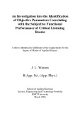
2.1b Real Critical Listening Room Measurements – Reverberation Time

Comparison:

The measurements in the field were very similar by design to those outlined

above. The same measurement signal chain was used. Additionally, the same software

and analysis method was used wherever possible. There was a method presented in the

Figure 2.2: Reverberation Times Critical Listening Room I

Reverberation Times - Method Investigation Listening Room I - Linear Vertical Axes

RTA Rev Back R Spkr (s)

0.70

RTA Reverb Back L Spkr (s)

RTA Reverb L Spkr (s)

0.60

RTA Reverb R Spkr (s)

0.50

30ms Slices L Spkr (s)

30ms Slices R Spkr (s)

i

0.40

MLS N=18 8 Reps L Spkr (s)

MLS N=18 8 Reps R Spkr (s)

0.30

IRS N=16 L Spkr (s)

IRS N=16 R Spkr (s)

) s ( e m T n o i t a r e b r e v e R

0.20

0.10

Sine Sweep Crossed Over L Spkr (s) Sine Sweep Crossed Over R Spkr (s) Sine Sweep Full Range L Spkr (s)

Sine Sweep Full Range R Spkr (s)

0.00

31.5

125

250

500

1000

2000

4000

8000

16000

Octave Frequency Band (Hz)

Reverberation Times - Method Investigation Listening Room I - Log Vertical Axes

1.00

RTA Rev Back R Spkr (s)

RTA Reverb Back L Spkr (s)

RTA Reverb L Spkr (s)

RTA Reverb R Spkr (s)

30ms Slices L Spkr (s)

30ms Slices R Spkr (s)

i

MLS N=18 8 Reps L Spkr (s)

0.10

MLS N=18 8 Reps R Spkr (s)

IRS N=16 L Spkr (s)

IRS N=16 R Spkr (s)

) s ( e m T n o i t a r e b r e v e R

Sine Sweep Crossed Over L Spkr (s)

Sine Sweep Crossed Over R Spkr (s)

Sine Sweep Full Range L Spkr (s)

Sine Sweep Full Range R Spkr (s)

0.01

31.5

125

250

500

1000

2000

4000

8000

16000

Octave Frequency Band (Hz)

Laboratory Methods that was not implementable in the field. The method refered to as the

‘Decay Quality Measured – AS1045’ (AS1). This method requires dedicated

instrumentation that wasn’t able to be installed in the critical listening rooms under test

here. Basically, the instrumentation quantifies the curvature of the decay measured and

rejects decays that are too curved.

For these measurements, the microphone was initially placed in the aural sweet

spot. Additional measurements were also performed at other locations around the room

and will be discussed further in the next chapter as will the differences between left

speaker and right speaker excitation. The data presented in Figures 2.2 and 2.3 are

averages of the data at the listening position and show the agreement between the

different methods. At this juncture, the researcher decided to survey two aurally distinct

critical listening rooms rather than one. The reasons for this were to verify the methods

under test in critical listening rooms that were considered to be subjectively different by

the researcher. It was hoped the objective data should broadly reflect these differences.

The researcher’s impressions regarding aural variations in critical listening rooms

were generally associated with the geometrical arrangement of the walls of the critical

listening room. Loosely speaking, there seemed to be two distinct types of critical

listening rooms: parallel wall floor plan (i.e. square or rectangular floor plan) and non-

parallel floor plan (rectangle with rounded corners floor plan, triangular floor plan etc).

Each broad geometrical category also could be broadly associated with their ‘sound’. To

illustrate, imagine two rooms are constructed with roughly the same volume and

reverberation time but with the geometrically different floor plans discussed above.

Speaking very generally, the researcher would describe the ‘sound’ of a rectangle floor plan listening room as ordered. The ‘sweet spot’ is focused around the central axis8

of the room. The off-axis response of the speakers is governed by the visual proximity of

room boundaries and, for want of a better description, walls sound like walls and corners

sound like corners. More technically, the degree of aural liveness of the room matches the

visual cues with respect to reflective surfaces. A non-parallel floor plan critical listening

room sounds much more diffuse and less ordered. The sweet spot is often amorphous in

8 The central axis: The axis halfway between the monitors/speakers running perpendicularly down the room.

shape with the sharpness of the stereo image not necessarily directly related to the central

axis of the room. The off-axis response of the speakers is again governed by the

proximity of the room boundaries. More technically, the room sounds more diffuse in

association with non-parallel geometrical arrangement of the room boundaries and

reflective surfaces.

It was desired to examine the measurement and analysis methods for repeatability

in the sweet spots of these two geometrically different critical listening room designs:

rectangular floor plan and non-rectangular floor plan. For these measurements, Critical Listening Room 1 is the approximately 35m3 room and features a non-parallel wall

Figure 2.3: Reverberation Times of Critical Listening Room II

Reverberation Times Method Comparison - Method Investigation Listening Room II - Linear Vertical Axes

0.80

0.70

0.60

0.50

0.40

0.30

) s ( e m Ti n o i t a r e b r e v e R

0.20

0.10

0.00

RTA RevBack R Spkr (s) RTA RevBack L Spkr (s) MLS N=16A sing Lspkr (s) MLS N=16A sing Rspkr (s) MLS N=16A 8reps Lspkr (s) MLS N=16A 8reps Rspkr (s) MLS N=16B, sing Lspkr (s) MLS N=16B, sing Rspkr (s) MLS N=16B 8reps Lspkr (s) MLS N=16B 8reps Rspkr (s) MLS N=18 sing Lspkr (s) MLS N=18 sing Rspkr (s) MLS N=18 8reps Lspkr (s) MLS N=18 8reps Rspkr (s) IRS L Spkr (s) IRS R Spkr (s) 30ms Slices L Spkr (s) 30ms Slices R Spkr (s) Sine Sweep Crossed Over L Spkr (s) Sine Sweep Crossed Over R Spkr (s) Sine Sweep Full Range L Spkr (s) Sine Sweep Full Range R Spkr (s)

31.5

125

250

500

1000

2000

4000

8000

16000

Octave Frequency Band (Hz)

Reverberation Times Method Comparison - Method Investigation Listening Room II - Log Vertical Axes

1.00

(

i

0.10

s) me Ti n o at r e b r e v e R

0.01

31.5

125

250

500

1000

2000

4000

8000

16000

Octave Frequency Band (Hz)

arrangement whilst Critical Listening Room 2 is also about 35m3 in volume and features

parallel walls. Both rooms sounded relatively dead. The researcher’s impressions of the

rooms were that they both ‘sounded’ good but were different in the ways described in the

previous paragraph. Brief discussion will be made later in the next section in outlining the

differences in the measured data in conjunction with the researcher’s informal

impressions. In line with accepted research practices and ethical considerations, the

researcher is not considered a subject of the research and consequently, no effort was

made to investigate objectively any of the researchers’ subjective or perceptual

impressions.

In the field, the in-situ monitoring equipment installed into the critical listening

room was to be used to excite the room. The room under test was excited using all of the

test stimuli in one speaker (say L) and then the other (say R). This resulted in two

measurements for each position. From a research perspective, this was desirable as when

the research program moves into the field, data will be taken for each of the monitor

speaker positions highlighting any acoustical anomalies in the room and/or monitor

position/mounting associated with excitation from different sides. These anomalies can

then be discretely measured. In most of the research, two microphones were used and so

each play of the stimulus resulted in four ‘independent’ microphone positions. The term

‘independent’ in this case is meant to mean the microphones were separated by a distance of λ/2 at the lowest frequency of interest. This was not always possible as functional

critical listening rooms can be quite small: often smaller in major dimension than the

half-wavelength of the lowest frequency being judged. Care was taken to ensure that the

most well separated microphone positions were chosen and any compromised positions

were appropriately noted. For the comparison presented here, 2 independent positions

(one pass of the stimulus) were possible but a total of 4 were taken in each room. These

were then treated as statistically independent results and were considered with this in

mind.

Getting enough energy into all of the bands of interest for all of the measurement

methods under test was a problem particularly with pseudo-random noise methods. The

test signals were generated and presented unaltered. They were not equalized or

manipulated in any way as these problems were not anticipated. However, these problems

have been encountered before with respect to pseudo-random noise methods. Pre-

emphasising the problem bands has been explored (Rife, D. D., & Vanderkooy, J., 1989)

but was not attempted here. For the purpose of these comparison tests, the solution to the

problem was simple. For the pseudo-random noise stimuli, the in-situ volume of the

driving loudspeakers was increased with great care to allow measurement across all of the

frequency bands of interest. It was not possible however to achieve desirable signal to

noise ratio in the low frequency bands for the pseudo-random methods all of the time.

The low frequency data was consequently accepted as not being as accurate.

As is evident from Figures 2.2 and 2.3, the different methods when measuring

reverberation times in the two critical listening rooms compare well in the higher

frequency bands and not so well in the lower frequency bands as is expected. The data

found in Figure 2.2 and 2.3 is presented in full in Appendix I in Table AppI6 – AppI10

and Table AppI11 respectively.

2.2 Evaluations of the Salience of the Objective Measurement Methods

The different methods were assessed on a repeatability and accuracy basis. Firstly

though, it is worth commenting on the results and methods more generally. As presented

above, all of the methods yielded comparable data for reverberation times. That said, it is

appropriate to specifically cite some of the procedural basis for the measurement and

analysis methods looked at here.

Fairly early on in considering the benefits and differences between the

measurement methods, it was established that the impulse response measurement

methods were most advantageous. This was due to the fact that the impulse response of a

room, once accurately measured, can be analyzed in many different ways to yield useful

data both in the temporal and frequency domains. This has the added benefit of the

researcher not having to specify precisely the analysis method on the fly. The research

was then able to proceed minimizing the limiting decisions being made regarding the

analysis of the impulse response data. The researcher was able to identify particular areas

of interest and process the data to examine the area of interest at any stage as the research

proceeded. And further, should there be a desire to alter the analysis method, it was then

not necessary to revisit any of the rooms measured as part of the research.

The repeatability of the measurements both in the field and in the laboratory was

found to be very good. In the laboratory, the measurements were repeated several times

using all of the methods under test and were found to vary little. The variation that was

observed was the lower frequencies where modal considerations would cause a degree of

physical variability in the results. The variability of results was considered acceptable.

The results of the measurements in the reverberation chamber are depicted in Figure 2.4

below (the results in their entirety appear in table form in Appendix 1 in Table AppI1 –

Table AppI5) and are simply averaged values of 4 repetitions of the measurement with

the 95% confidence interval calculated and depicted on the chart as y-axis error bars.

Figure 2.4: Repeatability Data: Reverberation Chamber with Error Bars

Repeatability between Different Methods- Reverberation Time Measurment Performed in Reverberation Chamber

9.00

8.00

7.00

Manual Slice Method Average (s)

6.00

5.00

i

Automated RTA Function Average (s)

4.00

Aurora Swept Sinusoid Method Average (s)

) s ( e m T b r e v e R

3.00

2.00

Aurora MLS Method Average (s)

1.00

0.00

31.5

125

250

500

1000

2000

4000

8000

16000

Octave Frequency Band (Hz)

The repeatability in the field was also investigated. The agreement between

different methods in the laboratory and the field was confirmed as reported above. The

repeatability investigations were not repeated in full in the field, mainly due to the time

consuming nature of some of the measurement methods. Since the agreement in the

measured reverberation times between the different methods was good in the field, it was

decided that the repeatability need only be verified for one of the field methods. The

repeatability of the impulse response methods was confirmed in Critical Listening Room

1 (see Figure 2.5, Appendix 1 Table AppI6 – AppI10). Again, the comparability between

the methods was very good. Similarly, the repeatability was also found to be very good.

Each of the methods was performed 4 times in each position with excitation coming from

both speakers.

Figure 2.5: Repeatability Data with Error Bars performed in Critical Listening Room 1

Reverberation Times - Repeatability Aurora Methods Performed in Critical Listening Room 1

0.80

0.70

0.60

Reverberation Time Swept Sine (60sec, 200Hz crossover) - R spkr (s)

0.50

i

0.40

Reverberation Time Swept Sine (60sec, 200Hz crossover) - L spkr (s)

Reverberation Time MLS Average R Spkr(s)

0.30

) s ( e m T b r e v e R

0.20

Reverberation Time MLS Average L Spkr (s)

0.10

0.00

31.5

125

250

500

1000

2000

4000

8000

16000

Octave Frequency Band (Hz)

Initially, positions measured in the sweet spot of the individual room were

compared to positions measured outside of the sweet spot. A total of 8 positions were

measured in Critical Listening Room 1. The comparison was performed to examine if

there seemed to be different measured reverberation times and acoustical parameters in

the two noticeably different perceptually and spatially listening positions in an individual

room (see Figure 2.6). Unfortunately, no useful patterns in any of the measured acoustical

parameters were noticed at this early stage in the research.

Figure 2.6 - Variation of Reverb Times as a function of Position

Reverberation Times - Critical Lsitening Room 1 (Sweeps)

0.60

0.50

Reverb Time Average All Positions (s) Pos 1

Pos 2

0.40

Pos 3

Pos 4

Reverberation Times – Critical Listening Room 1 (Sweeps)

i

0.30

Pos 5

) s ( e m T b r e v e R

Pos 6

0.20

Pos 7

Pos 8

0.10

0.00

31.5

125

250

500

1000

2000

4000

8000

16000

Octave Band Centre Frequency (Hz)

The comparison investigations implied that, for the majority of the rooms, a range

of pseudo-random noise samples and swept sinusoids would yield the desired objective

data. The use of these stimuli meant that large amounts of data could be collected in a

relatively short period of time with the different methods serving as confirmation of

accuracy. The pseudo-random noise featured a spectrum compatible with true random

noise. So, assuming the duration of the pseudo-random noise is sufficient to achieve

steady state in the room under test, the pseudo-random noise bursts could be treated as

interrupted noise allowing the direct measurement of the reverberation time (and EDT)

and a further avenue of comparison between methods if desired. This was also useful as

the other pseudo-random noise and swept sinusoid methods involved the mathematical

process of convolution and de-convolution as part of the extraction of the impulse

response. Various checks were necessary to ensure these processes were computed

correctly and were not found to be without their difficulties in implementation. This will

be expanded upon in the next chapter.

Another benefit of the impulse response objective analysis methods is their

portability. Put simply, the general analysis procedure can be applied to any part of the

signal chain. Thus it was envisaged, that if deemed necessary as the research proceeded,

it would be possible to measure the impulse response of aspects of the electro-acoustics

equipment in addition to the superimposed room acoustical and electro-acoustic

measurement.

2.3 Other Considerations for the Implementation of the chosen Objective Method in

the Field

The critical listening rooms which the researcher was keen to include in the

research were commercially operating critical listening rooms. Thus the objective

measurement had to be quick and easy to implement and non-destructive to the in-situ

monitoring system. It is appropriate to highlight at this stage that several other issues

were worth considering for field implementation of the methods discussed above. For

‘Surround’-style critical listening rooms, where there are 4 or 5 or more speakers, all of

the discrete speakers were to be used to excite the room individually. Obviously

particular attention is paid to the main left and right speakers as these are the speakers

common to other critical listening rooms designed to work with stereo and generally are

the ones most used for critical aural decisions in surround facilities. The presence of the

extra speakers was still considered relevant as all of the speakers in a surround-sound

equipped critical listening room contribute to the judgment sound field and consequently

we would like to measure any associated acoustical anomalies. An analysis of the sweet

spot as excited by different surround-speakers was considered outside the boundaries of

this research since the different specifications of the different speaker sends amongst

other relevant considerations would have to be considered. Such an analysis would

require a dedicated measurement procedure and was considered diversionary from this

research.

A range of factors affect the functional perceptual performance of the critical

listening room: aesthetics, monitor quality, environment, mood of subject, room

acoustics, etc. All of these factors play a role in the functional performance of a critical

listening room and for the purpose of these objective comparison tests, a positive

subjective appraisal from a professional listener was deemed sufficient for useful

objective comparison despite the quantitative variability of the other relevant subjective

and objective factors. Basically, the critical listener/proprietor responsible for the

acoustics of the facility in question has successfully adjusted a large range of inter-related

factors in achieving acceptable functional performance of their critical listening room.

The research featured here is primarily concerned with any linking parameters between

these objective and subjective components of critical listening rooms and thus the

researcher considered this level of functionality, only as an affirmative opinion of the

critical listening professional, to be of basic importance in the qualification of a listening

room as functional and further for the qualification for participation in this research.

2.4 Perceptual Aims and Considerations

Considered for implementation as part of the perceptual parts of this research

were neural networks, multi-variate analysis and various other statistical methods of

treating the subjective responses. The requirements associated with the implementation of

such methods included a degree of subject education, a large time commitment from the

subject, difficult logistical issues in controlling variables between subjects and various

bureaucratic ethical issues. Basically, these statistical analysis methods and their

associated data collection techniques were discarded as they were simply too hard to

implement.

The preliminary subjective investigations were to be performed in the ‘home’

studio of the critical listener subject. In this sense, ‘home’ means the studio in which the

subject is used to working professionally. The purpose of this was to ensure that the

listener was familiar and comfortable with the sound field quality in his or her room.

Similarly, they were familiar with the electro-acoustics of the room and the operation of

the electro-acoustics to respond subjectively and objectively to what they hear. Also,

many critical listeners have remarkable abilities to hear deficiencies in a critical listing

room and consciously compensate for these deficiencies in making critical aural

decisions. Ideally, the subjective aspects of this research would document these qualities

that are common amongst professional critical listeners.

Having identified a critical listener group and some of their common traits, it was

then a matter of finding a way to target the listener group and analyze the subject(s)

through the introduction of some sort of stimulus. The research program was intended to

look at some more complicated aural stimulation and examine the degree and quality to

which the stimulus response of the subject can be analyzed to provide useful information.

In an attempt to objectify perceptual feedback from the subject. We were interested to see

if it was going to be possible through a combination of objective and subjective

techniques to elicit useable perceptual data through the treatment of the subjects’ hearing,

aural processing and resultant response as a ‘black box’. We were presenting the subject

with a sound and looking at their response to the sound without any interest in how or

why they responded to the sound in the way they did. If we did happen to elicit a

perceptual response which was interesting, then it would be further investigated. In the

early stages of the subjective side of the research we were assessing if complicated

stimuli could be presented to a subject and yield useful data, and to investigate the level

of repeatability of the tests.

Having broadly decided on the intended nature of the subjective side of the

research, it was then appropriate to become more specific in the investigations. Firstly, a

range of stimuli was considered. Since the test subjects were professional listeners, it was

initially decided to attempt to find stimuli that would minimize subjective responses to

the stimuli themselves. Thus the stimuli would have to be as non-descript as possible: the

subjects should be familiar with the sound. To put it another way, in an attempt to

minimize these subjective responses, we wanted to find and present a ‘bread and butter’

sound to the subjects. To take a step back, if we consider a sound as presented for

judgment by a critical listener, the ‘pure’ sound is affected by a complicated

superposition of the electro-acoustics and acoustics of the recording and performance

room in both the temporal and frequency domains. Thus we were looking to present a

sound which was as ‘pure’ as possible: minimally effected by the method and

environment in which it was recorded. Thus it was decided to present common

instrument sounds which were recorded using an instrumentation grade microphone in an

anechoic chamber. The sounds had to have a ‘natural’ sound meaning that it had to sound

like a stereotypical version of the common instrument. The sound also had to be recorded

such that there was minimal frequency or dynamic alterations due to the recording signal

chain. Also the recorded noise floor had to be less than that of the recording studios so

that the subject only hears the noise floor of the recording studio. This is the noise floor

for which the subject is accustomed and so to alter the noise floor (or ‘silence’ for that

particular critical listening room) in any way would immediately introduce anomalies in

the subject’s appraisal of the sound and their critical listening room performance in

reproducing the sound. Also it was desired to arrange the presentation of the sound to the

subject to be as close as possible to the presentation that they would get in a real

recording session. It was envisaged that some editing of the sourced sounds might be

necessary to facilitate this type of presentation with the template for the presentation

based on the researcher’s experiences as a musician and audio engineer. The most

applicable anechoic sounds found were sourced from Behringer Audio Company entitled

‘Behringer Audio CD Vol 1: Our Own Way Reference CD’ (Behringer, 1999). Other

well known anechoic recordings were also sourced: ‘Music For Archimedes’ (Bang &

Olufson, 1992) and ‘Anechoic Orchestral Music Recording’ (Denon, 1988). These

recording were not used for various reasons. With both of the Denon and Bang &

Olufson recordings, the performances of the instruments mainly consisted of pieces of

music played by string instruments. The Behringer selection was much more broad and

included more contemporary instruments such as synthesizers.

In a real recording session, many subjective aural decisions are made by the audio

engineer through repetitive performance of the instrument being judged. Pieces of music

generally have to be editied, if such an edit is possible, to achieve such repetition. The

Behringer anechoic samples were already edited in this way. Much time would have been

necessary to edit the other recording into such a form. Also Archimides and Denon didn’t

have as wide a selection of percussion instruments as the Behringer recording.

Once appropriate sounds had been sourced, it was envisaged that these sounds

would be recorded onto a common medium with maximum quality for reproduction in

the critical listening room under test. The media with the anechoic sounds was passed to

the subject and they set up the room for listening as they would when normally doing

critical listening. To be clear, the subject controls the volume and playback of the

stimulus. It is appropriate to re-iterate that the subjects will be very used to the electro-

acoustics and acoustics of their own critical listening rooms.

The subject was then asked to ‘mix’ the stimuli. In this case ‘mix’ means to

prepare the sound both technically and subjectively to their satisfaction. The subjects had

access to both the temporal domain and the frequency domain to alter the sound and also

could optimize the performance of their listening facility by positioning themselves

where they are most comfortable making listening decisions and listen at a volume

entirely of their own choice. The context of the presentation of the stimuli (order, relative

volume, repetition, duration of particular sample etc) meant that the selected sounds

would be presented in a standard order and frequency similar to that of a recording

session. For example, the drums would be agglomerated as they would be if an engineer

was setting up to record a drum kit. Thus all of the audio microphones on the drum kit are

individually appraised and then frequently the instrument as a whole is checked for tonal

and dynamic balance: the engineer is ‘pulling’ a sound. Generally, each of the

instruments will be prepared and critically appraised as a discrete series of critical

listening decisions. Finally, all of the critical listening decisions made until that point will

be summed up into a single critical listening decision compiling the final program master

often called the program decision or final mix.

To summarize, we presented the subject with a series of recorded instrumental

sounds and got them to mix them. Given that we knew any of the measurable quantities

of the ‘raw’ unmixed sounds, we were interested in comparing these qualities to the

‘mixed’ sounds. At this early stage in the research, the attitude was to try a few things and

see if these attempts yielded any interesting observations worthy of further investigation.

So the analysis methods implemented initially were quite broad. As the human hearing

organ processes aural stimulus in both the temporal and frequency dimension, so the

analysis and comparisons of the data obtained by these tests would be analyzed to

examine any changes from the unmixed sounds in the temporal and frequency domains. It

was envisaged that the identification and quantification of any of these changes, when

compared to the objective room (and electro-acoustical) analysis data, might imply a

relationship of some sort between the subjective changes made to the sound as altered by

the environment in which it is presented and the objective quantification of that

environment.

2.5 Summary

For the objective room acoustic analysis, impulse response measurement methods

were identified as being the most appropriate for the research. For the subjective aspects

of the research, a range of anechoically-recorded stimuli were used. It is appropriate to

note that many aspects of the subjective research were going to remain unquantified. The

human listening organ was treated as simply a black box to see if there was any pattern in

the listeners’ responses; particularly when considered in conjunction with the results of

the objective room acoustic analyses.

3 Experimental Methodology in the Field

With respect to the objective measurements, the aims were clear. To measure, as

accurately as possible, the acoustical characteristics of the critical listening room under

test.

For the subjective aspects of the research, the initial aim was simply to mimic as

closely as possible a ‘real’ critical listening session. It was then hoped that the analysis of

the subjective data would reveal perceptual patterns that could be linked to objective

parameters measured in the room acoustic aspects of the research. Care was taken to

ensure that the subjects participated in the research under conditions entirely under their

control. This included all of the variables associated with critical listening including

volume of program, positioning in relation to monitoring etc. The only input from the

research was the provision of the sounds or stimuli to mix.

3.1 Objective Methodology and Instrumentation Limitations

It was desirous to standardize as much as possible all aspects of the objective

measurements. In the early stages of the performance of the research, extra time in each

of the critical listening rooms was allocated to perform measurements using several of the

impulse response measurement methods previously mentioned. The reasoning was

essentially that in the early stages of the research it was not known completely which of

the methods was easiest to implement and further how to derive the desired information

from the measurement. Also, the different methods suffered various distortions and time-

invariance problems to varying degrees. Thus there was significant interest in the

agreement and repeatability between the different methods. Of primary importance to all

objective measurements of acoustics in the field, the accuracy of the instrumentation

formed a large part of the initial considerations of the implementation of the

measurement. Keeping in mind that the pseudo-random noise techniques are extremely

dependent on the time invariance of the system under test, it was first checked that the

measurement instrumentation was time invariant. As a start, it was decided to check the

entire signal chain. The most likely place that time variance was possible in the

measurement signal chain was in the analogue to digital conversions. And for this reason,

the number of digital to analogue conversions (and vice versa) was kept to a minimum.

There are two conversions to consider: the conversion from digital to analogue of the

stimulus and the conversion from analogue to digital of the received microphone signal

for storage and post-processing. We could test the time invariance of the measurement

digital to analogue converters through simply playing the stimulus out of the line output

into the line input of the field signal storage unit. In this case, the field storage unit was a

DAT recorder. The stimulus was recorded onto the DAT tape at standard levels and then

processed to develop an impulse response. If the system as measured was time invariant,

the resultant impulse response will be a delta function: basically a pulse of infinite height

and infinitely short duration. In this case, the pulse magnitude will be the same magnitude

as the input and the pulse length is equal to 2 samples. It is appropriate to note that the

research DAT tape was ‘played’ into a PC for analysis but stayed in the digital domain

minimizing the potential for time jitters and errors.

A perfect impulse response is presented in the top image in Figure 3.1. The

horizontal axis is time and the vertical axis is relative level. Given the nature of the

deconvolution process, the ‘perfect’ impulse response as measured implies that the

system through which the impulse response was measured is time-invariant. Thus the

signal chains of relevance could be examined for time invariance using similar

measurement and analysis criteria. The middle image in Figure 3.1 shows an impulse

response with an introduced time variance. And finally, the bottom image was measured

using the digital output of the field DAT. For the first field measurements, the digital

output of the field DAT was used. Consequently, the transfer from the field DAT into the

PC for deconvolution and analysis introduced much error.

Access to another DAT player was facilitated and the digital output was

measured. This digital output proved to introduce no time errors and so was implemented.

The impulse response data for the investigation of the time invariance of the DAT used in

the research is presented in Figure 3.2. The frequency response of the DAT at 48 kHz

sampling frequency was also examined. Pink noise was recorded into the DAT player

using the in-built Analogue to Digital converters and played back into an analyser

capable of running 96 kHz sampling. This data is presented in Figure 3.3.

Figure 3.1: Measured Impulse responses of the digital to analogue conversion processes. Horizontal axis is time.

-1dB

-∞dB

-1dB

-∞dB

-1dB

-∞dB

-1dB

Fig. 3.2: Impulse response through the DAT player used in the research

-1dB

-∞dB

-1dB

Figure 3.3: FFT measurement of Pink Noise Played out of a standard DAT Player – Top diagram log horizontal axis, bottom diagram linear horizontal axis.

Another significant consideration in the implementation of the objective analysis

in the field was the choice of microphone. Since we were interested in all of the audible

frequency bands, we similarly were interested in implementing a microphone allowing

true measurements from 20 Hz to 22000 Hz. As a slight aside, the highest frequency of

interest, 22000 Hz was set not by some arbitrary research decision but is more associated

with the sampling rates available for use in the research. Compact discs and most non-

linear based sound editors have sampling rates of 44,100 Hz sampling rates. Thus due to

the Nyquist roll-off associated with digital sampling, the maximum frequency able to be stored on a CD or recorded using a DAT player or a non-linear sound recorder9 with a

sample rate of 44100 samples per second is 22050 Hz. As a result, our stimulus was

limited to a highest frequency of 22000 Hz due to the storage medium. A standard CD

player was checked to see if there were other frequency considerations in the CD

playback/reproduction process. Pink noise was generated digitally and recorded onto a

CD. The CD was then played into a FFT analyser to examine if there was an anti-aliasing

filter across the CD output. The FFT of the measurement constitutes Figure 3.4. As is

evident from the frequency response, there is a high frequency roll-off commencing at

approximately 19000 Hz. Thus our measurements from CD based stimuli will be limited

to frequencies below 19000 Hz.

9 A non-linear recorder is a disk based recording system allowing immediate access to any part of the program material.

Figure 3.4: FFT measurement of Pink Noise Played out of a standard CD Player – Top diagram log horizontal axis, bottom diagram linear horizontal axis.

For the purpose of measurement, the field DAT that was utilised was capable of a

48000Hz sample rate. This sampling rate was implemented in the field so as to maximize

the resolution of the higher frequency data as measured through the microphone signal

chain. Microphones were selected to be as flat as possible over the frequency bands of

interest. It is also appropriate to note that the sound-fields at the higher frequencies were

altered by the presence of the microphone itself. This is due to the wavelengths at the

higher frequencies being dimensionally comparable to the microphone itself. This led to

1/8 inch microphones being used in the research as these were the smallest microphone

able to be accessed for the research. The directional nature of the microphones was

considered but was not thought to be of significance to the placement of microphones

during research. Essentially, it was just a matter of getting enough energy into all of the

bands of interest so that the signal to noise ratio of the resultant impulse response was

optimized.

After having briefly discussed some of the frequency-based limitations of the

compact disc medium, it is now appropriate to outline the generation and sourcing of the

stimulus signals. As has already been stated, the stimulus signals, which were used to

measure the objective qualities of critical listening rooms, were those which were

analyzed to obtain the room/electro-acoustics impulse response. These signals were the

maximum length sequences, inverse repeated sequences and swept sinusoids. It was

ascertained from each of the critical listening rooms participating in the research which

format was the easiest to play through the in-situ speaker system(s). Thus the stimuli

were created as both a data file and CD format as required.

Figure 3.5: Noise floor of measurement signal chain - GRAS Mic, Pre and Power Supp. Recorded to DAT

Noise Rating Chart

90.0

80.0

70.0

)

Ch A

Ch B

60.0

50.0

B d ( l e v e L

NR 30

NR 40

40.0

e s i

30.0

o N

20.0

NC-25

NC-30

10.0

0.0

31.5

62.5

125

2000

4000

8000

250 1000 500 Frequency (Hz)

It was also desired to examine the noise floors of the various rooms. Several

instrumentation related considerations immediately became relevant. Firstly, the noise

floor of the instrumentation had to be measured. The graph of these measurements is

presented in Figure 3.5. The measurements were taken in a reverberant chamber with the

same signal chain as was used in the field. The chains were calibrated as per usual then

the noise floor of the reverberant chamber was recorded onto a DAT tape. The

measurements were linearly averaged samples of 2 minutes and 30 seconds. It was

thought that the acoustical noise floor of the Reverberant Chambers would be lower than

the noise floor of most of the critical listening rooms which might participate in the

research. And further, due to the small dimension of the microphone, it was expected that

the microphones, and consequently the measurement signal chain, would have significant

noise. Thus the measurement presented here can be called a background machine noise

measurement or the noise floor of the measurement signal chains.

As is evident from the chart in Figure 3.5, the microphone noise is significant. It

is equivalent in noise level to NC 25 and NR 40. This made it impossible to measure the

noise floors of most of the rooms slated to participate in the research. As there is already

much research on the effect of noise on critical listening and psycho-acoustics, it was

decided to continue with the 1/8 inch microphones and eliminate background noise in

critical listening rooms as an avenue of investigation in this research. Note that the

microphone/pre-amps/power supply front-ends were the noisiest part of the

measurement/analysis signal chain and hence this was the measurement noise floor for all

of the measurements.

Ultimately, the research gravitated towards implementing only the swept

sinusoidal methods in the objective analysis as we were reliably able to get good signal to

noise ratios in all of the bands of interest and the levels required did not worry the

critical listen room user/proprietors. The sinusoidal methods had several technical

advantages. The technique does not assume linearity and time invariance of the system

under test and was logistically easy to implement. Additionally, as the work of

(Vanderkooy, 1994) has shown with respect to pseudo-random noise techniques,

distortion artifacts present in either the measurement or excitation signal chains can result

in false reverberation measurements and spurious reflections in the measured impulse

response. The work of (Muller, S. & Massarani, P.,2001) has provided further arguments

for the implementation of swept sinusoids in this research as their work highlights the

significantly higher immunity against distortion and time variance than other techniques.

Also the work of (Farina, 2000) shows, swept sinusoid techniques allow easy further

analysis of any part of the signal chains should the need arise whilst conducting the

research. The use of the swept sinusoid techniques offered the additional advantage that

the distortions in the reproduction system were directly measurable and quantifiable if

required.

It should be noted that the measured impulse responses will be the superposition

of the transfer functions of all of the measurement and excitation signal chains’ transfer

functions. Should the research lead to more focused investigation of any particular part of

the signal chains exciting the critical listening rooms under test, then the methods and

instrumentation selected for use in the research should be appropriate for these further

investigations. It was also realized that it might be necessary to further check technical

aspects of the measurement signal chain in a similar way as we have examined the chain

for the room acoustical measurements presented in Chapter 2. These checks would

confirm the suitability of the research instrumentation for appropriate resolution in the

time and frequency domain.

3.3 Subjective Methodology in the Field

With the philosophy of trying to stay as close as possible to the logistical

and temporal aspects of a typical recording session, there were many considerations in

commencing the subjective investigations. The research was mainly concerned with

investigating professional critical listeners’ responses to complicated sounds. The

research aural program itself was also structured so that the repetition and duration of the

sounds was compatible to that in a real aural decision situation.

The audio engineer selected to participate in the preliminary investigations was a

experienced professional audio engineer with professional recognition from his peers.

The room in which he was to perform the preliminary listening tests was the room

extensively objectively analysed and reported in section 2.1b Real Critical Listening

Room Measurements – Reverberation Time Comparison and referred to as Critical

Listening Room 2. The objective aspects of the room were well known before the

commencement of the listening tests.

3.4 Summary

A template for the investigations of the objective characteristics of critical

listening rooms is presented. Incorporating a range of logistical and physical

characteristics of critical listening rooms, the method was engineered to be easy to

implement, of short duration and provide the least restrictions in analysis. The methods

implemented in the field were initially pseudo-random noise and swept sinusoidal tones.

These were stored on a medium compatible with the critical listening room under test for

excitation of the room through the in-situ monitoring system. As much data as was

logistically possible was taken in the maximum number of statistically independent

microphone positions to compile the objective analysis of the critical listening room

under test. These methods were compared using a loaded (reduced reverb time ~3s @

100 Hz, ~0.8s @ 8000 Hz) reverberant chamber and two critical listening rooms for both

agreement between methods and repeatability. For technical reasons, the chosen objective

room excitation stimuli ended up being exclusively swept sinusoids.

Further particulars for investigations in the subjective domain were also

presented. It is worth mentioning that the subjective areas of the research were very broad

in scope with further research being guided more or less completely by the results of

preliminary investigations. Consultation with external psycho-acoustic expertise was

considered outside of the scope of the research.

4 Results and Discussion

Having decided on and de-bugged the methods of objective analysis for this

research, the techniques were implemented over a period of three years in a range of

suitable critical listening rooms. These rooms all met the criteria of a critical listening

room as outlined in the previous chapter but were still widely varied in their particular

design. This observation was the basis for the structure of the analysis of the

measurements. The data was analyzed to look for variations in the temporal and

frequency domains. Since contemporary listening room/studio design criteria such as

Reflection Free Zone (RFZ) or Live-End-Dead-End (LEDE) (Davis 1980) designs place

such a large emphasis on the control of reflections, it was also decided to attempt to

investigate the time domain in some way different to decay analysis. Loosely, RFZ rooms

are exactly as they imply: the listening position is in a reflection free zone. There is no

time of arrival of reflections in theory. In the case of LEDE designs, there is a prescribed

time of arrival for the first reflections in the control room which physically depends

primarily on the dimensions of the control room in relation to the performance space in

which the program was recorded. Loosely speaking, the inspiration for the design derives

from the desirability of reflected sound arriving in what is commonly referred to as the

Haas Zone (Haas 1961). Reflected sounds arriving in the Haas Zone (reflections arriving

within ~50ms after the direct and sound with a relative intensity of roughly equal to the

direct wave) are thought to be perceived more pleasantly than sounds arriving outside of

the Haas Zone (<~20ms – the reflection is integrated by ear into the direct sound,

>~50ms the reflection is perceived as distinct from the direct sound). This perceptual

effect is also known as the Haas Effect or the precedence effect and describes the human

psychoacoustic phenomena of correctly identifying the direction of a sound source heard

in both ears but arriving at different times. The analysis of the impulse response also

allowed time of arrival of discrete reflections to be quantified. Through filtering the

impulse response, the room decay could be further quantified providing time-of-arrival

data as a function of frequency should the investigations warrant.

4.1 Impulse Response Notes

For most of the rooms measured, two impulse responses were generated for each

microphone-speaker position. This was due to the fact that two sweeps were implemented

to cover all of the frequencies of interest. Figure 4.1 depicts a high frequency and a low

frequency impulse response for one of the participating critical listening rooms and is

presented to simply show what the three typical IRs used in the research looked like . The

vertical axis is amplitude or level whilst the horizontal axis is the time axis. Also

presented is an IR as measured from a full-range sweep. The three IRs are completely

discrete in that they were measured separately. They were measured one after another

using the same instrumentation and mic position. As is evident from Figure 4.1, the

responses look similar.

Figure 4.1: A Standard Impulse Response – The top diagram is measured from a low frequency sweep (20Hz – 250Hz), the middle diagram is high frequency sweep (125Hz – 20000Hz) and the bottom diagram is a full range sweep. Major horizontal divisions 0.02sec

-1dB

-∞dB

-1dB

-∞dB

-1dB

-∞dB

-1dB

One immediately noticeable difference is that the low frequency impulse response

seems to persist for a longer duration than the other comparable diagram, the full range

sweep data. The reason for this slightly misleading depiction is that the impulse responses

were normalized10 to -6dB upon processing. Thus the vertical scale in the diagrams is not

identical and consequently direct comparison of the amplitudes between the impulse

responses presented in Figure 4.1 is not possible ie comparison of the visible tails. The

normalization was performed to maintain a good signal to noise ratio in the recovered

impulse responses. It should also be noted that the normalization process alters the

depiction of vertical axis and thus makes ‘events’ more prominent in the time domain and

could consequently prove misleading. For a few of the rooms, the main methods used for

the room analysis for this research were run in parallel with a time delay spectrometer.

Direct comparison between the methods is difficult due to the fundamental differences

between the techniques both in terms of their excitation and also the type of data yielded

from the application of the methods. The main benefit of time delay spectrometry is the

ability to measure particular acoustical events. The ease with which the instrument can be

set to do such measurements is essentially what gives it its advantages. Compatible

measurements using swept sinusoidal methods are possible but very difficult to

implement. Computer code would need to be written to introduce the appropriate time

delays and filters onto the measurement signal chain using constant percentage bandwidth

to allow the filtering out of all of the room acoustical reflections except for the reflection

being studied as the stimulus tone moves upward in frequency. If we set up the TDS

instrument to not apply any filtering or delay to the measurement signal chain then we get

a similar measurement method to those instituted as part of this research. Since the

instrument lacks the appropriate deconvolution and convolution tools, the researcher was

not able to find a way to perform a useful comparison between the methods investigated

as part of this research and time delay spectrometry.

4.2 Noted Non-Acoustical Characteristics of Critical Listening Rooms

The rooms that participated in this research varied in volume from approximately 16m3 to 175m3. A total of 17 rooms were measured. As much as was practical, the

dimensions, floor plan and a series of digital images were taken of the critical listening

rooms should the information be of use as the research progressed. The images also

10 Normalised to -6dB in this sense means that the recovered impulse responses were processed so that they all had a peak of -6dB.

recorded microphone positions and any other features of interest such as monitor

mounting or position of dedicated absorbers. The information on the geometrical layout

of the critical listening room allowed rough computation of path-lengths for the different

orders of reflection. This information could be correlated with time-of-arrival information

should the research demand. Also archived with each measurement was the temperature

and relative humidity of each of the rooms measured.

Absorption is commonly engineered into critical listening rooms. Notes on the

position and composition of any absorption material were recorded. This information

could be correlated with microphone positions giving an idea of some of the local

acoustical effects contributing to the resultant sound field in the listening position. Also a

feature in many critical listening rooms is dedicated diffusers. These are particularly

common on the back wall of the studio. Again, their presence was noted. Broadly, it was

anticipated that a particularly diffuse room as observed by the researcher could warrant

analyzing the measured impulse responses slightly differently as the research progressed.

Dedicated measurements of diffusion were considered too logistically difficult

(D’Antonio P., & Konnert K.,1992) and consequently beyond the scope of this research.

Many critical listening rooms have been designed following the LEDE or RFZ

critical listening room/studio design philosophies. Also monitor manufacturers such as

Genelec and Westlake recommend certain room acoustical characteristics to varying

degrees of specification (Varla, A., Mäkivirta A., Martikainen I., Pilchner M., Schoustal

R. & Anet C., 1999; Westlake, 2004). Any information regarding acoustical designs of

this nature was of primary interest to this research. Accordingly, if the critical listening

room owner implemented or is aware of any design philosophy inspiring or influencing

the room design then this was also noted down.

4.3 Measured Acoustical Parameters

As would be expected, the reverberation time for all 17 of the rooms was

measured and is

presented in Figure 4.2.

Figure 4.2: Reverberation Times of all critical listening rooms measured – top chart linear vertical axis, bottom chart logarithmic vertical axis

Also presented, in

Figure 4.3, is the Early

Decay Time (EDT) for

Reverb Times in Octave Bands - All Rooms, Swept Sine Method (Linear Vertical Scale)

0.90

0.80

all 17 of the rooms.

0.70

Much research has

0.60

been done into these

i

0.50

areas particularly in the

0.40

acoustical assessment

0.30

of concert halls and

) s ( e m T n o i t a r e b r e v e R

0.20

opera houses (Barron

0.10

0.00

1993; Beranek, 2004;

125

250

500

1000

2000

4000

8000

16000

Beranek, 1962 amongst

Octave Frequency Band (Hz)

many others). As is

evident from Figure 4.2

Reverb Times in Octave Bands - All Rooms, Swept Sine Method (Logaritmic Vertical Scale)

(Logarithmic Vertical Scale)

1.000

and 4.3, there is rather

large variation across

all of the rooms

measured. Given the

i

rather large variation in

design of the rooms to

be surveyed this is not

) s ( e m T n o i t a r e b r e v e R

unexpected. This is

0.100

also explained by

125

250

500

1000

2000

4000

8000

16000

pointing out that the

Octave Frequency Band (Hz)

rooms had a varying

amount of acoustic treatment as part of the design or commissioning of the functional

critical listening room.

As far as the data

Figure 4.3: Early Decay Times (EDT) of all critical listening rooms measured - top chart linear vertical axis, bottom chart logarithmic vertical axis

presented in Figure 4.2 and

4.3, there really aren’t any

Early Decay Times in Octave Bands - All Rooms, Swept Sine Method (Logaritmic Vertical Scale)

(Linear Vertical Scale)

1.00

0.90

striking features to discuss.

0.80

Table 4.1 features a table

0.70

of standard deviations

) s ( e m

0.60

i

across all of the rooms as a

T

0.50

function of frequency.

y a c e D

0.40

0.30

Essentially, we see a

y l r a E

0.20

0.10

variation in both the

0.00

125

4000

8000

16000

500

1000

measured reverberation

times and early decay times

250 2000 Octave Frequency Band (Hz)

compatible with the

variations in the volumes

Early Decay Times in Octave Bands - All Rooms, Swept Sine Method (Logaritmic Vertical Scale)

(Logarithmic Vertical Scale)

1.00

of the rooms surveyed. It is

also appropriate to note

that the rooms also can be

) s ( e m

categorized as being

i

T

0.10

compliant with the rather

y a c e D

loose recommendations in

y l r a E

(AS3) AS2107- 2000:

0.01

125

250

500

1000

2000

4000

8000

16000

Acoustics – Recommended

Design Sound Levels and

Octave Frequency Band (Hz)

Reverberation Times for

Building Interiors. The standard prescribes mid-frequency reverberation times and

background noise levels. For critical listening rooms, referred to in the standard as music

studios, the standard prescribes a mid frequency reverberation time chart as a function of volume with the minimum specified volume approximately 40m3. The specified mid- frequency reverb time for a 40m3 music studio is 1.2s. All of the rooms easily met this

recommendation. The background noise level for music studios is recommended to be

30dB(A) max. As the measurement instrumentation is noisier than the noise floor of the

spaces being measured, background noise was not measured. It is worth noting however

that the noise floor of the instrumentation is lower than the recommended noise level for

critical listening rooms in AS2107. Thus we can surmise that the rooms comply with the

noise levels recommended in AS2107.

The standard deviation presented in Table 4.1 shows averaged Reverb Times and

EDT times for all of the rooms. For the purpose of this exercise, all of the impulse

responses measured in the sweet spot were considered simultaneously (a total of 34 IRs).

The data exhibits a larger deviation across the rooms in the lower frequencies. This is to

be expected in line with the variation across the volume of the rooms. The variations in

the higher frequencies is much smaller. This is to be expected due to the acoustical

functionality engineered

Table 4.1: Standard Deviation for all rooms as a function of frequency

into the rooms. A large

reverberation time in a

Std Dev (RT60)

Frequency (Hz)

stereo listening room

will make it difficult to

discern and manipulate

the stereo image

(Gilford, 1979). Thus

the high frequency

attenuation present in

RT60 Average of All Rooms (s) 0.46 0.40 0.31 0.23 0.20 0.19 0.19 0.19 0.18 0.15

0.17 0.09 0.10 0.06 0.06 0.05 0.06 0.06 0.05 0.04

EDT Average of All Rooms (s) 0.40 0.36 0.26 0.24 0.20 0.17 0.18 0.16 0.16 0.14

Std Dev (EDT) 0.13 0.20 0.11 0.08 0.07 0.07 0.08 0.06 0.06 0.07

31.5 63 125 250 500 1000 2000 4000 8000 16000

all of the rooms is evident in the fast decay times as defined by reverberation time and

EDT. Essentially, the data implies that there is little general variation across the rooms in

the higher frequencies and that each individual sweet spot IR can be treated as a member

of an ensemble incorperating all of the sweet spot IRs as an ensemble.

Also measured was Clarity 50msec (C50), Clarity 80msec (C80), Definition

(D50), Centre Time (Ts), Tonal Balance (TB), Bass Ratio (BR), Treble Ratio 2000

(TR(EDT)2000) and Treble Ratio 4000 (TR(EDT)4000). The data generated was in

octave bands as well as linear and A-weighted data. The critical listening rooms under

test varied significantly (the data is presented in Appendix I in full). Due to the

interrelated nature of the parameters, it is not worth discussing them extensively in an

individual sense. In lieu of such discussion and mindful of the parameters’ inter-

relationship, correlation coefficients were calculated over the measured parameters. It is

worth briefly discussing in a broad sense the use of correlation in this particular case. For

the analysis to be quantitatively valid, a correlation analysis should be derived from

random measurements. These measurements are also supposed to follow a normal

distribution. It is quickly evident that this assumption is not generally adhered to and thus

the following results must be considered a qualitative indicator of mutual dependence of

parameters.

Firstly, it was decided to examine the correlation between individual parameters

(Pelorson et al 1992) as a function of speaker excitation. Table 4.2 and 4.3 features

correlation figures between all of the parameters for the parameter treating L speaker

excitation and R speaker excitation as mutually exclusive measurements. This statistical

investigation is meant to compliment the Decay vs. Frequency investigation presented

perviously and further imply the ensemble nature of the IRs and their independence of

side of excitation. For the purpose of the statistical comparison, the particular data which

was correlated was 500 Hz data for EDT and RT. The linear data was used to compare

the other acoustical parameters. Should these correlations show any interesting feature,

then the octave data would be examined for any other useful further analysis.

This statistical analysis was performed to see if there was any correlatable pattern

developed between comparing the parameters measured through the in-situ monitoring

system in an individual, Left and Right, sense. If there was no demonstrable correlation

then the implulse responses from the Left speaker and the Right speaker could be treated

as statistically independent data doubling the number of impulse responses to further

analyse in the relevant data set. Table 4.4 presents the correlation between L and R

particularly.

Table 4.2: Correlation Matrix - L speaker excitation

Volume

C50

C80

D50

Bass Ratio

Tonal Balance

Reverb Time

Early Decay Time

Treble Ratio 2000

Treble Ratio 4000

1

0.69

1

-0.55

Reverb Time Early Decay Time C50

1 -0.94

-0.57

C80

0.99

1 -0.94

-0.71

0.79

0.78

D50

1 -0.93

0.50

-0.70

-0.67

-0.89

0.80

1

-0.02

0.43

0.31

-0.38

1

-0.01

-0.12

0.04

-0.01

0.32

0.19

-0.33

0.34

0.09

Treble Ratio 2000 Treble Ratio 4000 Tonal Balance Volume

1 Table 4.3: Correlation Matrix - R speaker excitation

C50

C80

D50

Volume

Reverb Time

Bass Ratio

Tonal Balance

Early Decay Time

Treble Ratio 2000

Treble Ratio 4000

1

0.37

1

Reverb Time Early Decay Time C50

-0.19

-0.92

1

C80

-0.89

-0.15

0.30

-0.36

Treble Ratio 2000 Treble Ratio 4000 Tonal Balance Volume

0.02

0.05

-0.03

-0.10

0.09

-0.14

0.24

0.25

-0.19

0.38

1 Table 4.4: Correlation Matrix - L vs, R speaker excitation

Reverb Time L

Early Decay Time L

C50 L

C80 L

Bass Ratio L

Treble Ratio 2000 L

Treble Ratio 4000 L

Tonal Balance L

D50 L

Tc L

Volume

0.69

-0.89

0.80

-0.29

-0.06

-0.21

-0.37

0.02

0.97 -0.95

Reverb Time R Early Decay Time R

0.32

0.77

-0.18

-0.19

-0.37

0.21

0.36

-0.26

-0.52

0.33

0.05

C50 R

-0.53

0.78

-0.67

0.40

-0.11

0.27

0.49

-0.03

-0.92

0.97

C80 R

-0.89

-0.50

0.73

-0.61

0.37

-0.07

0.22

0.47

-0.10

0.94

0.96

D50 R

-0.88

-0.69

0.73

0.72

-0.86

0.23

0.14

0.29

0.09

0.98

0.88

0.66

-0.77

-0.75

-0.96

0.86

-0.29

-0.09

-0.17

-0.34

-0.14

-0.38

-0.02

0.49

0.47

0.35

-0.33

0.79

-0.10

-0.04

0.84

0.32

0.00

0.11

-0.08

-0.10

0.14

-0.05

-0.15

0.48

0.16

-0.08

0.19

-0.23

-0.47

0.08

0.13

0.01

-0.54

0.37

0.42

-0.47

-0.33

Tc R Bass Ratio R Treble Ratio 2000 R Treble Ratio 4000 R Tonal Balance R

-0.45

-0.07

0.45

0.46

0.34

-0.28

0.75

-0.07

-0.25

0.85

0.34

Volume

0.09

-0.01

-0.12

0.04

-0.01

0.40

-0.30

-0.33

0.45

1

It is worth expanding on some

points about calculation method with

respect to the ISO3382 parameters.

Given the similarities in the

calculation between D50 and Ts, a

should short Ts measurement

correspond with a high D50

measurement. Table 4.5 contains the

D50 and Ts broadband measurements

for the averaged values for left and

right as measured in the listening

position. The values have been

ranked from lowest D50 to highest.

As is evident from the data, the

lowest D50 values correspond to the

highest Ts time. Given the variation

in the geometric shape and the

absorption/diffusion in the critical

listening rooms, the variation in the

data was not considered to be unusual.

Keeping in mind that C50 is thought to be representative of the clarity of speech

and C80 is thought to be representative of the clarity of music, it was thought that the

difference in C50 and C80 might yield some interesting data. The methods of calculation of C50 and C80 involve the integration of the p2(t) signal over the first 50msec and

80msec respectively. Thus the data can be considered to be measures of the proportion of

energy arriving before 50msec (C50) and 80msec (C80). Thus further, it was thought that

it would be advantageous to examine this data for each of the two main

Figure 4.4: Energy Ratio of C50 and C80 Comparison – All rooms

Clarity Comparison Chart - All Rooms

40.0

35.0

30.0

25.0

Average Speaker Ratio

20.0

Left Speaker Ratio

15.0

o i t a R ) 0 5 C 0/ 8 C ( y g r e n E

Right Speaker Ratio

10.0

5.0

0.0

10 11 12 13 14 15 16 17

Critical Listening Room

speakers. In the presentation of the raw data it is difficult to see any useful patterns: it is

just a bunch of numbers. Accordingly, it was decided to represent the data as a ratio

between C50 and C80 in the energy domain. To simply compare the data between rooms

tends to be futile due to the differences between the rooms and there being no direct way

to compare in this case. Using the ratio will yield proportional data between 50msec and

80msec in each individual room. The data which is presented in Figure 4.4 is a function

of left and right speaker as measured in the listening position. The average of left and

right is also presented.

Figure 4.5: Treble Ratio 2000Hz and 4000Hz Comparison Chart

Difference Chart: (TR(EDT)2000-TR(EDT)4000)

0.400

0.300

0.200

0.100

TR(EDT) 2000 - TR(EDT) 4000 (Right Speaker)

0.000

-0.100

TR(EDT) 2000 - TR(EDT) 4000 (Left Speaker)

-0.200

-0.300

-0.400

-0.500

Critical Listening Room

In a general sense, the comparison between the left and right speakers shows the

performance of most of the rooms to be essentially acoustically symmetrical. And further

provides support to the acceptability of treating all of the IRs as an ensemble. It is evident

from Figure 4.4 that some of the rooms were more lively on one side than on the other.

Of particular interest is the general observation that the higher ratios are from right

speaker excitation in rooms where there was a significant difference between left and

right speakers. Further, the taller bars imply a larger proportion of the energy arrives after

50ms.

Figure 4.6: Bass Ratio and Tonal Balance Comparison Chart

0.50

0.40

0.30

BR - TB (Left Speaker)

0.20

0.10

BR - TB (Right Speaker)

0.00

-0.10

-0.20

-0.30

-0.40

10 11 12 13 14 15 16 17

(BR-TB) Difference Chart: (BTR-TB)

Critical Listening Room

Other acoustical parameters were also calculated: Tonal Response (TR), Bass

Ratio (BR), Treble Ratio – 2000 Hz (TR(EDT)2000) and Treble Ratio – 4000 Hz

(TR(EDT)4000). The data is presented in full in Appendix I. Considering the method of

calculation for the bass ratio and the tonal balance (see 1.4 Method of Analysis of

Objective Data) and the actual data upon which it is based (reverberation times and early

decay times), the parameters serve to offer a more focused objective link between

temporal and frequency considerations in room acoustics. From consideration of the

methods of calculation of these parameters, it is implied that these parameters might be

best considered as related pairs: TR and BR as the first pair and the two Treble Ratios as

the second pair.

Figure 4.7: Tonal Balance Left and Right Comparison Chart

Comparison between Left and Right Speaker - Tonal Balance (TB)

3.00

2.50

2.00

Tonal Balance (TB) - Left Speaker

1.50

1.00

Tonal Balance (TB) - Right Speaker

0.50

0.00

10 11 12 13 14 15 16 17

Critical Listening Room

Firstly, considering the methods of calculation of the Tonal Balance (TB) and the

Bass Ratio (BR) combined with the general observation that reverberation time decreases

as frequency increases we can then surmise that the TB can be expected to be less than

the BR. The other two acoustical parameters, TR(EDT)2000 and TR(EDT)4000, when

considered similarly imply that TR(EDT)2000 should be greater than TR(EDT)4000.

Interestingly, this was not always found to be the case in the measurements performed on

the rooms participating in this research. Broadly speaking, about half of the rooms

measured seemed to follow the expected trend whilst half did not (see Figures 4.5, 4.6,

4.7 and 4.8).

In the temporal domain, we were interested in quantifying the differences in the

time of arrival of different reflections. The time of arrival of the reflected energy after the

direct energy has been widely documented to be related to perceptual considerations

through such documented phenomena as the precedence effect (Haas, 1961; Wallach, H.,

Newman E.B. & Rosenzweig M.R., 1949) and temporal masking (Atal, Schroeder &

Kuttruff, 1962). In line with this, many of the room specifications for critical listening

such as the LEDE specifications previously mentioned or the BS775-1 (ITU 1992)

specifications have definite recommendations for the time of arrival of the first

reflections as well as specifications for the relative level of these reflections to the direct

energy. The impulse responses could be analysed to generate an energy time curve (ETC)

allowing the quantification of the time of arrival of the first reflection after the direct

sound and also to measure the relative levels between the first reflection and the direct

sound in the listening position.

Table 4.6: Table of Time of Arrivals and Relative Magnitudes for Right Speaker Excitation in the Listening Position

Critical Listening

Time of

Relative

Time of

Relative

Time of

Relative

Room

Arrival -

Magnitud

Arrival -

Magnitude -

Arrival -

Magnitud

Approximate Volume (m3)

1st

e - 1st

2nd

3rd

e - 3rd

Reflectio

Reflection

Reflectio

n (ms)

n to Peak

(ms)

to Peak

n (s)

n to Peak

2.8

0.06

6.8

0.12

14.4

0.09

6.8

0.32

15.8

0.24

26.2

0.12

3.6

0.32

7.6

0.17

15.7

0.14

175

4.0

0.67

17.3

0.34

34.3

0.15

4.3

0.61

7.8

0.60

10.2

0.54

11.9

0.32

13.0

0.23

20.7

0.20

3.3

0.39

7.9

0.43

8.8

0.48

1.8

0.43

3.5

0.49

4.9

0.66

6.7

0.64

14.7

0.71

41.3

0.60

5.2

0.38

9.4

0.43

10.9

0.36

1.7

0.63

6.0

0.48

28.0

0.40

1.5

0.61

5.4

0.42

36.3

0.47

2.8

0.55

4.6

0.66

6.5

0.48

4.0

0.60

7.3

0.60

17.9

0.45

1.3

0.56

2.7

0.54

4.7

0.39

3.3

0.62

4.6

0.68

7.9

0.40

2.0

0.52

4.1

0.67

6.5

0.57

Figure 4.8: Bass Ratio Left and Right Comparison Chart

Comparison between Left and Right Speaker - Bass Ratio (BR) Comp

2.50

2.00

1.50

Bass Ratio (BR) - Left Speaker

1.00

Bass Ratio (BR) - Right Speaker

0.50

0.00

10 11

13 14

16 17

Critical Listening Room

The data was plotted using linear scales on both the time and the energy axes. The

use of a logarithmic scale on the energy axis was also investigated. This was investigated

to ascertain if major acoustical events could be analysed and discerned with greater

resolution through depiction of the energy axis on a logarithmic scale. Finally, on the

suggestion of Kuttruff (Kuttruff, 1991), the formed and rectified envelope function from

the impulse responses were also convolved with a 25ms time constant exponential (y = e(1/0.025)) to mimic some of the time-based responses of the human ear. Consideration of

the ETCs, in conjunction with the EDT and reverberation time data, show that the rooms

could be characterized as ‘dead’.

Table 4.6 above catalogues variation across the rooms of the arrival of the first

‘major’ reflections at the listening position for excitation from the right speaker in all of

the measured critical listening rooms. In most of the rooms, the data for left speaker

excitation is very similar to that of the right speaker as would be expected. Consequently,

the discussion surrounding the data for the right speaker generally also has relevance to

the left speaker data. Objective examination and analysis of differences between left and

right performance of the critical listening rooms, which were surveyed using the ETC

data, was pursued and will be expanded upon in the next paragraphs.

Remembering that all of the measurements presented here were taken in the

listening position, the first reflection measured was considered to be the glancing

reflection off of the mixing desk. The glancing reflection from the mixing desk would

also be expected to have a similar path length to the direct signal which is evident in our

data both from an analysis point of view and through visual inspection of the energy-time

curves themselves.

The relative strengths between the direct sound and the major reflections were

also quantified. We would expect the relative magnitude to be similar between left and

right in association with the practical design criteria of acoustical symmetry of critical

listening rooms. Again, the expected similarities between left and right were evident. The

relative magnitude of the early reflections are also small. This support the broad

observation that critical listening rooms are subjectively ‘dead’ compared to ‘standard’

rooms. It was impossible to discern much more about the individual acoustic events as

the spatial layout of the critical listening rooms under test were not documented well

enough to allow for such judgments to be made.

The usefulness of the data would be increased through performing the

measurements using a Dummy Head. Echo-criteria and objective analysis procedures

similar to those proposed by Dietsch and Kraak (Dietsch and Kraak - 1986) and Niese

(Niese - 1961) can best be assessed through data taken in a dummy head. For these

reasons, more detailed analysis of the impulse responses was not undertaken unless there

was some impetus for further analysis through other areas of analysis and consideration

of the data. The relevance of the data with respect to certain more contemporary binaural

perceptual parameters (i.e. Inter Aural Cross-Correlation) and traditional methods of their

measurement was largely compromised. Basically, the identification and quantification of

reflections in studying the ETCs were judged subjectively by the researcher.

As the data in Table 4.2 shows, the time delays of acoustical events deemed

significant from the analyzed ETCs in no way approach 50msec. This might lead to the

observation that the critical listening rooms surveyed were designed so that all of the

significant room reflections arrive at the listener in the Haas Zone. This stands to reason

as a critical listening space with reflections arriving outside of the Haas Zone would be

perceived to have discrete reflections. The effect of this on critical listening decisions is

difficult to quantify as many competing temporal and frequency related perceptual effects

would be simultaneously occurring. The sum total of these competing perceptual hearing

effects would make the critical listening decisions made in such a room associated only

with that room. The mixed program played in any other room would be perceived

completely differently. Thus a critical listening room really must have certain acoustical

characteristics governed by the nature of hearing and the perception thereof. On a deeper

level, the arrival of these lateral reflections at times less than 50msec has a perceptual

auditory effect associated with the quality of the stereo image and the degree of comb-

filtering evident in the sound-field.

4.4 Case Study: Room 2

Room 2 Data – All measurements taken in Listening Position unless otherwise noted:

Table 4.7: Room 2 Left Speaker Acoustical Parameters ISO 3382

Left

Frequency

Left Speaker:

Speaker

Speaker:

(Hz)

Critical Listening

D50 (%)

C80(dB)

C50 (dB)

Critical

Room 2

Ts (ms)

Listening

Reverberation

Room 2

Time (s)

Early

Decay Time

(s)

0.48

0.32

18.0

21.4

98.4

46.1

31.5

0.30

0.20

16.5

19.6

97.8

31.7

63

0.23

0.19

20.7

35.0

99.2

19.1

125

0.15

0.13

18.3

26.6

98.6

18.1

250

0.14

0.12

22.1

40.1

99.4

6.9

500

0.13

0.10

28.0

43.7

99.8

5.8

1000

0.12

0.07

27.8

44.7

99.8

5.5

2000

0.14

0.08

23.9

41.7

99.6

6.7

4000

0.13

0.07

27.5

46.0

99.8

4.8

8000

0.12

0.05

31.3

47.8

99.9

2.9

16000

Table 4.7a: Room 2 Left Speaker Time of Arrival Data

Left Speaker: First Reflection

Left Speaker: Second

Left Speaker: Third Reflection

Time of Arrival (ms) ) -

Reflection Time of Arrival (ms)

Time of Arrival (ms) -

Broadband

- Broadband

Broadband

3.05

8.50

22.00

Table 4.7b: Room 2 Left Speaker Acoustical Parameters Non-ISO3382

Tonal Balance (TB) - Left Speaker

Bass Ratio (BR) - Left Speaker

TR(EDT) 4000 - Left Speaker

BR - TB (Left Speaker)

TR(EDT ) 2000 - Left Speaker

1.36

1.13

0.48

0.45

0.23

TR(EDT) 2000 - TR(EDT) 4000 (Left Speaker) 0.03

Critical Listening Room 2

Right Speaker Data: Table 4.8: Room 2 Right Speaker Acoustical Parameters

Right

Frequency

Right Speaker:

Speaker

Speaker:

(Hz)

Critical Listening

D50 (%)

C80(dB)

C50 (dB)

Critical

Room 2

Ts (ms)

Listening

Reverberation

Room 2

Time (s)

Early

Decay Time

(s)

0.47

0.30

9.4

14.4

89.7

65.8

31.5

0.32

0.20

10.9

19.6

92.5

41.8

63

0.24

0.20

20.1

29.8

99.0

24.1

125

0.15

0.14

22.2

25.6

99.4

16.5

250

0.14

0.11

26.9

51.0

99.8

8.9

500

0.13

0.11

24.3

50.9

99.6

6.7

1000

0.11

0.08

26.3

45.3

99.8

7.2

2000

0.12

0.09

25.0

41.2

99.7

7.5

4000

0.12

0.08

27.3

45.1

99.8

5.7

8000

0.12

0.06

29.9

48.7

99.9

6.0

16000

Table 4.8a: Room 2 Left Speaker Time of Arrival Data

Right Speaker: First Reflection

Right Speaker: Second

Right Speaker: Third

Time of Arrival (ms) -

Reflection Time of Arrival (ms)

Broadband

- Broadband

6.82

15.76

26.18

Table 4.8b: Room 2 Right Speaker Acoustical Parameters Non-ISO3382

Tonal Balance (TB) - Right Speaker

Bass Ratio (BR) - Right Speaker

TR(EDT) 4000 - Right Speaker

BR - TB (Right Speaker)

TR(EDT ) 2000 - Right Speaker

1.15

1.07

0.64

0.79

0.08

TR(EDT) 2000 - TR(EDT) 4000 (Right Speaker) -0.143

Critical Listening Room 2

Acoustical Parameters Both Speakers – Graph Format

Figure 4.9: Room 2 Reverberation time and Early Decay Time Data

Room 2 Data: Reverberation Times and Early Decay Times for Both Speakers

0.600

0.500

Left Speaker: Critical Listening Room 2 Reverberation Time (sec)

0.400

Left Speaker: Critical Listening Room 2 Early Decay Time (sec)

0.300

i

) s ( e m T

Right Speaker: Critical Listening Room 2 Reverberation Time (sec)

0.200

Right Speaker: Critical Listening Room 2 Early Decay Time (sec)

0.100

0.000

31.5

125

250

500

1000

2000

4000

8000

16000

Octave Frequency Band (Hz)

Figure 4.10: Room 2 Acoustical Parameters

Room 2 Data: C50, C80, R50 and Ts Both Speakers

100.0

90.0

Left Speaker C50 (dB)

80.0

Left Speaker C80(dB)

70.0

Left Speaker D50 (%)

60.0

Left Speaker Ts (msec)

50.0

y t i t n a u Q

40.0

Right Speaker C50 (dB)

30.0

Right Speaker C80(dB)

20.0

Right Speaker D50 (%)

10.0

Right Speaker Ts (msec)

0.0

31.5

125

250

500

1000

2000

4000

8000

16000

Octave Frequency Band (Hz)

Frequency Response and Smoothed ETCs for Room 2:

Left Speaker Excitation: Figure 4.11: Frequency Response for Critical Listening Room 2 – Left Speaker Excitation

Frequency Response Comparison - Left Speaker Excitation

-20

-40

)

B d ( l

-60

e v e L

-80

-100

-120

1346

2692

4037

5383

6729

8075

9421

10767 12112 13458 14804 16150 17496 18842 20187 21533

Frequency (Hz)

Figure 4.12: Smoothed Energy Time Curve for Critical Listening Room 2 – Left Speaker Excitation

Right Speaker Excitation:

Figure 4.13: Frequency Response for Critical Listening Room 2 – Right Speaker Excitation

Frequency Response Comparison - Right Speaker Excitation

-20

-40

)

B d ( l

-60

e v e L

-80

-100

-120

1465

2930

4395

5859

7324

8789

10254 11719 13184 14648 16113 17578 19043 20508 21973 23438

Frequency (Hz)

Figure 4.14: Smoothed Energy Time Curve for Critical Listening Room 2 – Right Speaker Excitation

Variation of Reverb Time in Different Microphone Positions:

Pos 1 (s)

Pos 2 (s)

Pos 3 (s)

Pos 4 (s)

Pos 5 (s)

Pos 6 (s)

Pos 7 (s)

Pos 8 (s)

Table 4.9: Variation of Reverb Time as a Function of Position – 4 individual positions, 2 excitation sources – in chart form

Frequ ency (Hz)

Reverb Time Average All Positions (s)

95% Confidence Reverberati on Time (s) 0.020

0.47

0.49

0.46

0.42

0.50

0.47

0.48

0.46

0.469

31.5

0.32 0.24 0.15 0.14 0.13 0.11 0.12 0.12 0.12

0.35 0.24 0.13 0.13 0.13 0.14 0.12 0.13 0.13

0.29 0.20 0.16 0.15 0.14 0.13 0.13 0.13 0.11

0.30 0.20 0.15 0.14 0.14 0.13 0.13 0.13 0.12

0.35 0.20 0.17 0.14 0.13 0.12 0.13 0.12 0.11

0.36 0.18 0.14 0.15 0.13 0.13 0.13 0.12 0.12

0.35 0.25 0.17 0.14 0.13 0.12 0.12 0.12 0.11

0.32 0.22 0.17 0.16 0.14 0.13 0.14 0.13 0.12

0.330 0.216 0.155 0.144 0.134 0.126 0.128 0.125 0.118

0.022 0.021 0.013 0.008 0.004 0.008 0.006 0.004 0.006

63 125 250 500 1000 2000 4000 8000 16000

Figure 4.15: Variation of Reverb Time as a Function of Position – 4 individual positions, 2 excitation sources – in graphical form

Reverberation Times as a Function of Position - Critical Listening Room 1

2

0.600

0.500

Reverb Time Average All Positions (s) Pos 1

Pos 2

0.400

Pos 3

Pos 4

i

) s ( e m T

0.300

Pos 5

b r e v e R

Pos 6

0.200

Pos 7

Pos 8

0.100

0.000

31.5

125

250

500

1000

2000

4000

8000

16000

Octave Band Centre Frequency (Hz)

Discussion:

Brief Description of Room 2:

Room 2 was a fairly new facility at the time of measurement. It is mainly intended

to work on stereo post-production programming. The electro-acoustics, whilst functional,

had really been simply placed with no real consideration of placement or mounting

conditions. The room acoustics could be described as a work in progress. The room had

parallel walls but a low ceiling that was not parallel to the floor. The ceiling was made

out of light building materials and had a hole cut into it. There was no conscious design

as far as the researcher could ascertain behind the structure/height of the ceiling. The

aesthetics of the room seemed to have come first: the room featured a couch against the

back wall and a series of drapes had been hung on the walls. There was also a small vocal

booth/performance room at one end of the room which had a glass window boundary.

The glass had been covered by a light blanket. Geometrically, the room featured parallel

walls (except for the ceiling) and was rectangular in shape. The major length dimension

was approximately 1.7 times the width dimension. The approximate volume of the room was 35m3. The monitors were installed at one end of the room. The studio owner was the

main user of the facility but it was also available to be hired out by free-lance engineers.

The facility was very busy with a range of professional, broadcast-standard projects.

Discussion of Results for Room 2:

The measured acoustical parameters for Room 2 are interesting from several

perspectives. The ETCs and the reflection analysis of the ETCs above show some

differences between left speaker excitation and right speaker excitation. Interestingly this is not obvious from the reverberation times. Since the room is approximately 35m3 in

volume, it is amongst the smaller facilities analyzed as part of this research.

Consequently, the times over which acoustical events occur are very short. The room was

set up with the monitoring mounted into the walls designed to radiate over and past a

computer screen. There was no mixing console in front of the operator/engineer. Instead

there was a keyboard and a range of analogue signal processing equipment favoured by

the studio owner/engineer. To the left of the engineer in relation to the monitoring, was

another rack of favoured processing equipment approximately 0.75m from the listening

position. On the right side was a CD rack approximately 2m from the listener. It is

thought that reflections from this rack are the later quite strong reflections seen on the

ETC for right speaker excitation for Room 2, see Figure 4.14. The higher clarity

measurements as a function of frequency for right hand speaker excitation also implies

the higher amounts of energy present from the reflections off the racks.

The variation of the reverberation times as a function of position (see Figure 4.15,

Table 4.9) was also very stable. The reverb times did not change significantly as a

function of room position. It is worth noting that the separation of the individual

measurement positions was limited by the size of the room. Thus the positions cannot be considered statistically independent in the 125 Hz, 63 Hz and 32 Hz octave bands11.

None-the-less the variation in the reverberation times around the room is very small.

The variations of the other acoustical ISO3382 parameters was also examined.

The measured variations are presented in Table 4.10 below.

Table 4.10: Mean Value Range (difference between the lowest and the highest measurement over all of the octave bands) and Standard Deviation as a function of position.

Acoustic Parameter Mean Range Value Standard Deviation

C50 3.67 1.82

C80 7.55 2.85

D50 0.40 0.16

7.37 2.54 Ts

Considering the method of calculation of the parameters, the variations observed

were to be expected. The mean value range is presented due to the low variation in the

reverberation times as a function of frequency when the measurements are performed at

different positions.

11 With the statistical independence of the positions decreasing with frequency.

4.5 Case Study: Room 6

Room 6 Data– All measurements taken in Listening Position:

Table 4.11: Room 6 Left Speaker Acoustical Parameters ISO3382

Left

Frequency

Left Speaker:

Speaker

Speaker:

(Hz)

Critical Listening

D50 (%)

C80(dB)

C50 (dB)

Critical

Room 6

Ts (ms)

Listening

Reverberation

Room 6

Time (s)

Early

Decay Time

(s)

0.48

0.36

14.3

22.6

96.4

52.2

31.5

0.36

0.29

8.8

13.6

88.4

38.1

63

0.30

0.24

16.8

22.8

97.9

26.6

125

0.21

16.6

24.2

97.9

11.8

250

0.19

0.18

16.2

23.9

97.7

13.1

500

0.22

0.19

15.3

23.7

97.1

10.3

1000

0.26

0.25

15.3

23.9

97.2

12.2

2000

0.25

0.23

16.9

24.8

98.0

9.2

4000

0.20

0.18

16.7

24.9

97.9

9.0

8000

0.18

0.17

19.3

27.9

98.8

8.4

16000

Table 4.11a: Room 6 Left Speaker Time of Arrival Data

Left Speaker: First Reflection

Left Speaker: Second

Left Speaker: Third Reflection

Time of Arrival (ms) -

Reflection Time of Arrival (ms)

Time of Arrival (ms) -

Broadband

- Broadband

Broadband

7.56

16.30

33.11

Table 4.11b: Room 6 Left Speaker Acoustical Parameters Non-ISO3382

Tonal Balance (TB) - Left Speaker

Bass Ratio (BR) - Left Speaker

TR(EDT) 4000 - Left Speaker

BR - TB (Left Speaker)

TR(EDT ) 2000 - Left Speaker

1.00

1.02

0.44

0.40

-0.02

TR(EDT) 2000 - TR(EDT) 4000 (Left Speaker) 0.042

Critical Listening Room 6

Right Speaker Data: Table 4.12: Room 6 Right Speaker Acoustical Parameters ISO3382

Right

Frequency

Right Speaker:

Speaker

Speaker:

(Hz)

Critical Listening

D50 (%)

C80(dB)

C50 (dB)

Critical

Room 6

Ts (ms)

Listening

Reverberation

Room 6

Time (s)

Early

Decay Time

(s)

0.39

0.38

9.1

12.0

89.0

69.1

31.5

0.36

0.31

6.7

12.5

82.5

49.2

63

0.29

0.23

0.22

15.3

23.7

97.2

10.5

8000

0.17

0.16

18.5

27.6

98.6

7.7

16000

Table 4.12a: Room 6 Right Speaker Time of Arrival Data

Right Speaker: First Reflection

Right Speaker: Second

Right Speaker: Third

Time of Arrival (ms) -

Reflection Time of Arrival (ms)

Broadband

- Broadband

11.93

13.00

20.67

Table 4.12b: Room 6 Right Speaker Acoustical Parameters Non-ISO3382

Tonal Balance (TB) - Right Speaker

Bass Ratio (BR) - Right Speaker

TR(EDT) 4000 - Right Speaker

BR - TB (Right Speaker)

TR(EDT ) 2000 - Right Speaker

1.11

1.08

0.62

0.68

0.02

TR(EDT) 2000 - TR(EDT) 4000 (Right Speaker) -0.059

Critical Listening Room 6

Both Speakers – Graph Format

Figure 4.15: Room 6 Reverberation time and Early Decay Time Data

Room 6 Data: Reverberation Timea and Eartly Decay Data - Both Speakers

0.5

0.45

0.4

Left Speaker: Critical Listening Room 6 Reverberation Time (sec)

0.35

0.3

Left Speaker: Critical Listening Room 6 Early Decay Time (sec)

) c e s (

0.25

i

Right Speaker: Critical Listening Room 6 Reverberation Time (sec)

e m T

0.2

0.15

Right Speaker: Critical Listening Room 6 Early Decay Time (sec)

0.1

0.05

0 31.5

125

250

500

1000

2000

4000

8000

16000

Frequency (Hz)

Figure 4.16: Room 6 Acoustical Parameters

Room 6 Data: C650, C80, R50 and Ts Both Speakers

100.0

90.0

Left Speaker C50 (dB)

80.0

Left Speaker C80(dB)

70.0

Left Speaker D50 (%)

60.0

Left Speaker Ts (msec)

50.0

y t i t n a u Q

Right Speaker C50 (dB)

40.0

Right Speaker C80(dB)

30.0

Right Speaker D50 (%)

20.0

Right Speaker Ts (msec)

10.0

0.0

31.5

125

250

500

1000

2000

4000

8000

16000

Octave Frequency Band (Hz)

Frequency Response and Smoother ETCs for Room 6:

Left Speaker Excitation:

Figure 4.17: Frequency Response for Critical Listening Room 6 – Left Speaker Excitation

Frequency Response Comparison - Left Speaker Excitation

-20

-40

)

-60

B d ( l e v e L

-80

-100

-120

1346

2692

4037

5383

6729

8075

9421

10767 12112 13458 14804 16150 17496 18842 20187 21533

Frequency (Hz)

Figure 4.18: Smoothed Energy Time Curve for Critical Listening Room 6 – Left Speaker Excitation

Right Speaker Excitation:

Figure 4.19: Frequency Response for Critical Listening Room 6 – Right Speaker Excitation

Frequency Response Comparison - Right Speaker Excitation

-20

-40

)

B d ( l

-60

e v e L

-80

-100

-120

1465

2930

4395

5859

7324

8789

10254 11719 13184 14648 16113 17578 19043 20508 21973 23438

Frequency (Hz)

Figure 4.20: Smoothed Energy Time Curve for Critical Listening Room 6 – Right Speaker Excitation

Discussion:

Brief Description of Room 6:

Room 6 was a state-of-the-art facility at the time of measurement. Designed to

work on stereo post-production programming, functionality to also operate as a surround-

sound facility was maintained though not central to the facility’s operation. The electro-

acoustics were extremely highly engineered and were amongst the most respected models

on the market. The monitors had been matched and were mounted according to

specification. The monitor system was verified for correct installation through successful

passing of the manufacturer’s criteria through objective testing. The room had passed

these tests and had been verified as within specification at the time of this research. The

exact specification was not available to the researcher as the test itself is of commercial

value to the monitor manufacturer. Also the rooms were not to be identified and the

mention of such a specification would serve to further identify the room. The room

acoustics were very highly designed with a number of dedicated diffusers mounted

throughout the room. Additionally, the rack-mounted gear was split into two racks found

on either side of the engineer. The room had a mixing desk installed in front of the

engineer. There was also a computer screen but this had been recessed into the same

mounting bench into which the mixing desk had been mounted. On the right side of the

engineer was a tape transport control. Although quite compact, the controller was of

significant size and would be expected to contribute to the sweet-spot sound-field due to

its proximity. The acoustical treatment appeared to be symmetrical about the central axis

of the room. The room also had a couch and a small machine room was attached. With

the studio in full operation, the machine room was completely inaudible in all parts of the

room. There was also an attached performance space with a window bordering between

the two spaces. The window was between the monitors and was not covered when the

room was in operation. It had been engineered into the acoustical performance of the

room. The majority of the time the room was used as a post-production facility and the

vision screen was accommodated over the window to the performance room.

Geometrically, the room featured parallel walls and was rectangular in shape and was of nominally the same volume as Room 2 discussed above: 38m3. The major length

dimension was approximately 1.3 times the width dimension. The monitors were installed

at one end of the room.

Discussion of Results for Room 6:

The measured acoustical parameters for Room 6 are interesting due to the fact that

they reflect the amount of acoustical and electro-acoustical engineering that has gone into

the design of the facility. The acoustical parameter data when compared between sides

varies little in line with the broad subjective observations made above by the researcher.

The frequency response and ETC data however do show some differences. The left

speaker excitation data shows more acoustical events in the ETC curves. It is thought the

very short reflection(s) would be due to the proximity of the tape transport controller. The

increased filtering is also thought to be due to the controller. It would be interesting to

measure the room again without the controller in position so as to confirm its contribution

to the measured sound-field in the listening position.

What variation there is between left and right manifests itself in the lower

frequencies. The differences are most obvious in the 31.5 Hz and the 63 Hz data. The

effect of modal behavior of rooms at these frequencies is demonstrated, as also seems to

be happening in all of the rooms, through the observed variation in the data at these

frequencies.

4.6 Other Statistical Analyses

Preliminarily, few other statistical investigations was performed. Essentially, the

purpose was to attempt to identify outliers in the data set. Any identified outlier could

then be further investigated or stripped from the data set as dictated by the research.

Informal appraisal of the data hints that there are no outliers to be stripped from the data

set. A more formalized method of outlier identification was instituted (Rousseeuw 1987,

Barnett et al 1984). The method identifies outliers using a modified z-test and is

summarized as follows:

In a modified z-score test the z-score is determined based on outlier resistant estimators.

The median of absolute deviation about the median (MAD) is such an estimator.

The MAD is calculated as follows:

MAD = median{|xi – xm|}

Where xi – value, xm is the sample median.

The MAD is calculated and used in place of standard deviation in z-score calculations.

The test heuristic states that an observation with a modified z-score greater than three and

a half should be labeled as an outlier. This is a reliable test since the parameters used to

calculate the modified z-score are minimally effected by the outliers.

The reverberation time (over both 20dB and 30dB decays) and EDT were

examined in this way in an attempt to identify outliers in the data. It was thought that an

outlier would become evident through failing the test presented above consistently across

all of the parameters tested. The results of the oulier identification tests are presented in

Table 4.13.

Table 4.13: Identified Outliers - RT and EDT

RT20 RT20 RT30 RT30 EDT EDT

L: R: L: R: L: R:

Outlier Critical

4,5, Listening Room

10 - - 10 9,14,16 8,9,12 Number

There was not enough consistency in the identification of any particular room as

an outlier to warrant it being left from the data set. Similarly, not one of the rooms

exhibited consistent oultlier status to warrant any type of dedicated investigation

objectively or otherwise.

The reverberation time and EDT data was also investigated using conventional

confidence limits. Confidence levels from 90% to 99% were calculated across all 17

rooms with 2 IRs/room included (total 34 IRs). The results are presented below in table

format in table 4.14 and 4.15. The third decimal place is presented to highlight the small

variations but is invalid in an empirical sense due to calculation and instrumentation

limitations.

Table 4.14: Reverberation Times compiled Confidence Limits - All Rooms

Frequ

90%

91%

92%

93%

94%

95%

96%

97%

98%

99%

Avera

ge of

Confiden

ency

All

ce - All

(Hz)

Rooms

0.464

0.068

0.070

0.073

0.088

0.081

0.085

0.090

0.096

0.107

0.075

31.5

0.399

0.037

0.039

0.040

0.048

0.045

0.047

0.049

0.053

0.059

0.041

63

0.305

0.040

0.041

0.042

0.051

0.047

0.049

0.052

0.056

0.062

0.044

125

0.225

0.024

0.025

0.026

0.031

0.029

0.030

0.032

0.035

0.038

0.027

250

0.199

0.023

0.024

0.025

0.030

0.028

0.029

0.031

0.033

0.036

0.026

500

0.191

0.022

0.023

0.028

0.026

0.027

0.029

0.031

0.034

0.024

1000

0.193

0.023

0.024

0.025

0.030

0.028

0.029

0.031

0.033

0.036

0.025

2000

0.192

0.023

0.024

0.029

0.027

0.028

0.030

0.032

0.036

0.025

4000

0.180

0.022

0.023

0.028

0.026

0.027

0.029

0.031

0.034

0.024

8000

0.152

0.024

0.025

0.026

0.031

0.029

0.030

0.032

0.034

0.038

0.027

16000

Table 4.15: EDT compiled Confidence Limits - All Rooms

Frequ

Avera

90%

91%

92%

93%

94%

95%

96%

97%

98%

99%

ge of

Confiden

ency

All

ce - All

(Hz)

Rooms

0.403

0.047

0.048

0.050

0.060

0.056

0.058

0.062

0.066

0.073

0.052

31.5

0.359

0.062

0.064

0.066

0.080

0.074

0.078

0.082

0.088

0.098

0.069

63

0.259

0.048

0.049

0.051

0.061

0.057

0.059

0.063

0.067

0.075

0.052

125

0.239

0.027

0.028

0.029

0.035

0.032

0.034

0.036

0.038

0.042

0.030

250

0.199

0.026

0.027

0.033

0.031

0.032

0.034

0.036

0.040

0.028

500

0.170

0.026

0.027

0.028

0.034

0.031

0.033

0.035

0.037

0.041

0.029

1000

0.177

0.026

0.027

0.033

0.031

0.032

0.034

0.036

0.040

0.028

As is evidenced by the table above, the observed variations across the critical

listening rooms is small in terms of decay rates. This stands to reason when considering

the design of critical listening rooms both intuitively and objectively (see Section 4.0).

4.7 Limitations of Objective Analysis

The main logistical limitation of the objective analysis was the available time

required for access to the space to be measured. Given the fact that the rooms were

working rooms, and rather than having an acoustical analysis performed they could be

earning money, the limits of time of access often shortened or abridged the analysis that

was possible.

It is also appropriate to note the limitations introduced in time/frequency domain.

The storage instrumentation has a sampling rate of 48 kHz with the consequent Nyquist

roll-off at 24 kHz. A few of the ‘higher-end’ rooms (essentially meaning more

expensive/higher quality electro-acoustics equipped rooms) surveyed as part of this

research informally claimed flat frequency response up to 50 kHz. It would be interesting

to examine these claims on a purely objective level and see how they alter from room to

room.

4.8 Outline of Subjective Investigations

The subjective investigations were undertaken fairly early on in the chronology of

the research. In a relatively short period of time, a great deal of data was able to be

generated which consequently was then time consuming to analyze. In the sections that

follow, the work is broadly outlined beginning with a description of the room in which

the subjective investigations were performed. Some demonstrative examples of the data

are also presented.

4.9 Summary of Objective Measurements of Room in which Subjective Research

was Performed

The critical listening room in which the subjective investigations were performed

was investigated extensively and referred to previously as Critical Listening Room 3. In

this section, the room will be broadly discussed with reference to all of the measured

acoustical parameters with special reference to its particular professional use and

functionality. It is hoped that this will give the reader an idea of the acoustical context of

the room in which the subjective investigations were performed.

Chart 4.21: Reverb times and EDT – Critical Listening Room 3.

Reverberation Time and EDT - Critical Listening Room 3

0.50

0.45

0.40

0.35

Reverberation Time - Ave (s)

0.30

0.25

i

) c e s ( e m T

0.20

EDT Ave (s)

0.15

0.10

0.05

0.00

31.5

125

250

500

1000

2000

4000

8000

16000

Frequency (Hz)

Critical Listening Room 3 was built in the 1970’s as part of an Audio Education

School. It was loosely designed to have non-parallel walls and was engineered to be relatively dead. The approximate volume of the room was 32m3. There were some

pseudo-Schroeder diffusers installed on some of the walls particularly the back wall

behind the listeners. There was also an adjoining performance room and accordingly, a

large window dominates one wall. The room is rectangular in shape with the shorter room

dimension being the direction of propagation of the monitoring (central axis was the

shorter dimension). There is a mixing desk and table in front of the listening position. The

desk/table would be responsible for the initial reflections depicted in the ETCs for Room

3 found in Figure 4.23. The facility is used mostly to record music and music-related

program for broadcast, advertising/marketing and mass production. The facility is

operated mostly by the owner (who in this case is the Subject) but is available for hire by

freelance engineers.

The data shows that the room is relatively true when excited by both the left and

right sides of the monitoring: it is acoustically symmetrical. On a more subjective level,

in the opinion of the researcher the room seemed to have a ‘boomy’ quality in the low

frequency bands. The researcher also felt that the left and right channels sounded quite

distinct and separated. When a sound was put down the centre, it sounded like it came

from left and right rather than from down the centre. The drop in the definition in the

lower frequencies and these resultant differences between left and right might be

responsible for this perceptual response from the researcher.

Figure 4.22: Acoustical Parameters for Critical Listening Room 3.

C50, C80, R50 and Ts as a Function of Frequency - Critical Listening Room 3

120

100

C50 Lspkr (dB)

C80 Lspkr (dB)

R50 Lspkr (%)

Ts Lspkr (msec)

C50 Rspkr (dB)

y t i t n a u Q

C80 Rspkr (dB)

R50 Rspkr (%)

Ts Rspkr (msec)

125

250

500

1000

2000

4000

8000

16000

0 31.5

Octave Frequency Band (Hz)

Figure 4.23: Smoothed Energy-Time curve for Critical Listening Room 3.

4.10 Some Initial Results of the Subjective Investigations

Essentially the subjective investigations never got past the initial investigation

stage. The first and only subject highlighted the complexity of the questions posed by this

research particularly when considering the role perceptual factors play in the assessment

of a critical listening room. The perceptual factors and the preferences of any individual

will vary across a group of people when considering any subjective and/or perceptual

auditory decision. Critical listeners and their objective and subjective preferences in

critical listening room characteristics are no different.

To briefly reiterate the nature of the investigations: the subject was presented with

a series of ‘common’ anechoic sounds and encouraged to ‘mix’ the sounds to taste in both

the time and frequency domain (see Section 2.4). The same subject was visited several

times with the same stimuli presented in different orders with different repetition

intervals but tending towards the general structure of a real recording or critical listening

session. The results of the mixing sessions were archived and examined through

producing spectrograms and waterfall diagrams of the original sounds and then the

‘mixed’ sounds. The subject was healthy over the course of the investigations.

Figure 4.24: Spectrogram and waterfall diagrams of anechoic kick drum

To commence the analysis phase of these preliminary investigations, the anechoic

stimuli were broken up into two categories: tonal and impulsive. Tonal anechoic sounds

consisted of instruments which were tonal in nature and featured a harmonic structure.

Some of the tonal instruments have an impulsive attack: i.e. plucking. The impulsive

sounds consisted of percussive and drum sounds. Generally speaking, to the researcher all

of the anechoic stimuli sounded quite unnatural with the special observation that the

impulsive sounds exhibited this to a greater degree.

Figure 4.25: Spectrogram and waterfall diagrams of ‘mixed’ kick drum – Session 1

It is thought that the hearing process is automatically analyzing the environment

in which the sound was recorded as part of the identification process applied to the sound.

Thus the dryness of the impulsive sounds was considered subjectively more anomalous

than the similar dryness associated with the tonal sounds.

A more general observation would be that the subject seemed to approach the

mixing of the tonal and impulsive sounds slightly differently. The tonal sounds were

more likely to be ‘mixed’ with delay/phasing type of effects applied. The impulsive

sounds were more likely to be ‘mixed’ with reverb effects. Due to the fact that the tonal

sound exhibited harmonic structure, it was surmised that the delay/phasing effects were

altering the harmonic balance of the sound in a way that was pleasant to the subject. The

Figure 4.26: Spectrogram and waterfall diagrams of anechoic snare drum – Session 1 and 2

impulsive sounds were more likely to be mixed using reverb effects to give the anechoic

samples a more natural sound: people generally don’t record or listen to anechoic spaces.

There were many ways in which the mixed data could be compared to the

anechoic samples. Of the graphical methods, spectrograms and waterfalls were obvious

choices for commencing to visually discern any patterns in the mixed sounds. Since both

generation of spectrograms and waterfalls involve fast Fourier transforms, this constituted

the main initial tool in analysis of the data. The well-known limitations of FFT (Stanley,

1984 amongst many others) was problematic in the lower frequencies of interest with all

of the sounds. Consequently the investigations at this preliminary stage were limited to

higher frequencies. At the higher frequencies (<400 Hz), there was thought to be no

technical limitation in the FFT analysis that would prevent some sort of

Figure 4.27: Spectrogram and waterfall diagrams of a mixed snare drum - Session 1

pattern from potentially being revealed.

The objective analyses of the mixed sounds yielded no identifiable patterns when

compared to the anechoic sounds. The choices the subject made in ‘mixing’ the anechoic

sounds to taste were not found to be characterisable in any way, let alone with respect to

any aspect of room acoustics. Examination of the spectrograms and waterfalls for the

Figure 4.28: Spectrogram and waterfall diagrams of ‘mixed’ snare drum – Session 2

kick drum and snare drum shows several important things. Firstly, whilst there are visible

graphical differences between complimentary sounds (see Figures 4.24 and 4.25 and

Figure 4.26, 4.27 and 4.28), in this case anechoic and ‘mixed’ sounds, the tests were not

found to be repeatable (Figures 4.27 and 4.28). After repeated tests, the critical listening

subject didn’t appear to produce a pattern of perceptual responses to the same stimuli.

The brief presentation of the anechoic sounds was not specific enough in its application

and inquiry. Also the complexity of the stimuli and the elicited subjects’ response led to

competing listening phenomenon making any degree of scientific repetition impossible

with the methods investigated here. Due to this preliminary result on a single subject, the

subjective investigations were not widened to include other critical listeners as it was

thought that the data would be similarly impossible to characterize in any useful way.

It was briefly considered that we attempt to alter the FFT analysis. Perhaps by

narrowing the frequency band of interest and tailoring the FFT parameters for the

frequency band we might yield some useful information or reveal some repeatability in

the data. This was not done as the investigations presented above gave no real direction

for such an analysis and the rigour of the method of investigation was objectively

dubious.

4.11 Variations in Subjective Investigations to Attempt to Yield Useful Data

Some slight variations in the procedure and stimuli involved in the subjective

investigations were investigated. A microphone was placed near the subject in the room

listening position whilst the subject ‘mixed’ the sounds to obtain an idea of the sound-

field as it was being manipulated by the subject.

The only pertinent observation to be made with respect to the data is essentially

confirmation of the complexity of the hearing process and response and the lack of rigour

in the measurement and analysis method when considered in conjunction with the

subjective investigation aims. The comparisons between all of the different sets of data

were initially analyzed to provide nominal frequency and time domain data. Firstly, the

identical tests participated in by the subject were compared for repeatability. Very

quickly it became evident that the basic initial analysis showed there to be differences

between the mixed data sets and consequent reinforcement for the lack of potency of the

method of investigation.

The room microphone signal was analysed in the time and frequency domain. As

one would expect, the analysis showed the superposition of the room acoustics with the

direct sound. Attempts were made to devise a method of analysing the data on deeper

level in an attempt discern any sort of pattern. Correlation and convolution methods were

considered to examine the differences between the ‘unmixed’ sound as stored on media

and the ‘mixed’ sounds as recorded during the mixing process through the microphone in

the sweet spot. There were several difficulties which were never resolved which

prevented any useful data being taken. Namely, the syncing of the sounds in the time domain was very difficult due to the instrumentation available for the research12. Aural

cues were considered but not implemented due to introducing anomalous sounds into the

investigation method in the presence of the subject. These difficulties are not

insurmountable and might be worthy of researching in future work assuming a suitable

analysis method can be devised to correlate the stimuli pair.

4.12 General Evaluation of the Results

The research shows objective variation in the measured acoustical parameters. For

example, the reverberation times for the range of critical listening rooms surveyed did not

seem to correlate to any particular trend in the objective domain outside of objective

trends associated with the physics of sound propagation in rooms as a function of

frequency. The rooms exhibited varying amounts of acoustical treatment in accordance

with the subjective preferences of the critical listener the room is designed to cater to.

Similarly, these variations can be extended to the monitoring systems and their

relationship to the acoustics of the critical listening room.

12 The syncing problems seemed to imply slight differences between the internal clocks in the A-D converters in the measurement DAT and the multi-track to which the mixed sounds were stored (evidenced by apparent delay increasing with elapsed time of session). The audio was judged by the subject after it had undergone this conversion. Investigation of this apparent delay was possible but considered outside the scope of this research.

Figure 4.29: A ‘dead’ room’.

Time (s)

In the lower frequencies, the rate of sound decay is slower. In critical listening

rooms, if there is an audible anomalous low frequency decay rate then it is common to

see these frequencies explicitly targeted for attenuation. The rooms measured all

exhibited a degree of acoustical treatment but the amount and effect of the absorption was

not explicitly investigated and was considered to be outside of the scope of this research.

One interesting aspect of the data was the fairly even decay rates found above 500 Hz. At

frequencies above 500 Hz, the reverberation time seems to asymptote to approximately

0.15s. In an aurally descriptive sense, the rooms were measured to be ‘dead’. To digress

slightly, the researcher found that the rooms didn’t sound excessively dead. The

researcher also made the subjective observation that there seemed to be a slight increase

in liveness at higher frequencies (roughly <1000 Hz). To a very slight degree the

reverberation time data (and confidence intervals ie increase in the confidence interval at

2000 Hz compared to 1000 Hz) supports this general observation but was not able to be

correlated in an objective sense. For example, the rooms were not categorized in the

objective sense such that it was possible to objectively investigate if there was a

relationship between this observed increase in the liveness/reverberation time at the

listening position and the positioning of racks of signal processing gear found in every

studio.

Figure 4.30: A ‘live’ room

Time (s)

The frequency response of the room’s monitoring was also measured. All of the

rooms exhibited degrees of comb filtering in the measured responses. Acoustical comb

filtering occurs when sound from a single source, such as a loudspeaker, is directed

toward a microphone or listener at a distance. The first sound to reach the microphone

will be the direct sound, followed by delayed reflected sound. Because the reflected

sound lags in phase relative to the direct sound, there will be cancellation at certain

frequencies where the two are 180 degrees out of phase, and augmentation at other

frequencies where the direct and the reflected sounds arrive in phase. Because it is a

function of wave length, the comb filter effect will notch out portions of the audio

spectrum at regular octave-spaced intervals. The subjective effect of comb filter effects,

is an added roughness to the sound, a reduction of harmonic richness and a smearing of

lateral stereo image focus and placement. An attempt to quantify the degree or depth of

100

Figure 4.31: Decay Time Comparison of ‘Boomy’ Room with the Average of all rooms

Decay Time Comparison of a 'Boomy' Room with the Average of All Rooms

1.00

0.90

Critical Listening Room 8 Early Decay Time (sec)

0.80

0.70

Average Early Decay Time of All Rooms (sec)

0.60

0.50

i

) s ( e m T

0.40

Critical Listening Room 8 Reverberation Time (sec)

0.30

0.20

Average Reverberation Time of All Rooms (sec)

0.10

0.00

31.5

125

250

500

1000

2000

4000

8000

16000

Octave Frequency Band (Hz)

comb filtering was not attempted. Consideration of monitor placement and mounting as

well as lateral absorption characteristics were not analyzed explicitly as part of the

research.

The other measured acoustical parameters, clarity (50 and 80), treble ratio (2000

Hz and 4000 Hz), bass ratio, tonal balance, definition and centre time. The parameters

were of use in determining the degree of acoustical symmetry achieved in the rooms. In

the case of C50 and C80, a degree of information in the time domain was measured

(defined at 50 ms and 80 ms respectively for the definition of clarity). As part of a

dedicated room analysis, these acoustical parameters allow quite good objective

characterization of the acoustical differences between rooms but could by no means be

considered comprehensive. There would be cases where rooms that are audibly different

have very similar measured acoustic parameters.

The major conclusions from the subjective data presented as part of this research

was that the interactions of the perceptual and objective acts of listening are very

complicated. There were too many unquantifiable variables interfering with any useful

objective patterns that might be able to be deduced from subjective listening tests.

Interestingly, a few of the rooms had obvious acoustical characteristics that seem to

dominate the ‘sound’ of the room. A basic characterization as a room being ‘live’ or

101

‘dead’ is very common. Figures 4.29 and 4.30 show smoothed13 energy time curves for

rooms which could be broadly described as live or dead.

Figure 4.32: Right Speaker Excitation ‘Boomy’ Room Impulse Response and ETC

Time (s)

13 The curve is obtained by convolving the envelope with a function designed to mimic the integrating properties of the ear, in this case exp(-t/time constant - here 25ms) (Kuttruff 1991).

102

The researcher also made some very informal subjective observations regarding the

sound of some of the rooms. One of the rooms, Critical Listening Room 8, would be

characterized by the researcher as excessively ‘boomy’. The room was quite elongated in

one dimension and had relatively little acoustic absorption in the space. The reverberation

time data and early decay time data reflects the boominess to a degree. Examination of

Figure 4.31 above shows the differences in the decay rates (specifically reverberation

time and early decay time) between the ‘boomy’ listening space and the average of all of

the rooms. Examination of the ETCs and the impulse responses themselves shows

anomalous features. When the impulse responses themselves are compared to a

‘standard’ impulse response such as that depicted in Figure 4.1, we can see that the tail of

the impulse is much longer indicating the presence of acoustic energy for a much longer

period of time in the latter more subjectively ‘boomy’ room.

The impulse responses and ETCs depicted in Figure 4.33 and 4.32 show the visual

characteristics in the objective data measured in a room broadly subjectively

characterised as ‘boomy’. A less ‘boomy’ room would have an impulse response which

has a shorter duration and decay particularly in the lower frequencies.

103

Figure 4.33: Left Speaker Excitation ‘Boomy’ Room Impulse Response and ETC

Time (s)

104

5 Summary and Conclusion

5.1 Objective Measurement Summary

The research was ambitious in its scope. As a result of this range of possibilities

and the unknown nature of what the final analysis methods might realistically entail, a

very large amount of data was taken. A large part of the research was the investigation of

a range of techniques suitable for performing the research. These techniques were both

subjective and objective in content and prospective outcome with the investigations

geared towards identifying the techniques which would be most likely to yield useful

information in the direction of the objectives of the research. Whilst there were aspects of

success with respect to investigating some of the available objective room analysis

techniques, the broader objectives of the research were far more elusive. The linking

parameters between subjective and objective functionality in critical listening rooms are

difficult and complicated to investigate. It is hoped that aspects of the work performed

here will aid future researchers in structuring their work so that it is more likely to lead to

an objectively demonstrable outcome. The researcher certainly gained significant insight

into the relationship between objective and subjective factors involved in critical listening

room design whilst performing the research. The insights though are subjective in essence

and personal in application. The difficulty, as is evident from the research performed and

reported here, is quantifying an aspect of critical listening room design which is

scientifically repeatable as a nominal linking parameter in either or both of the subjective

and objective domains.

Due to the broad research topic, it was desirable to select an objective

measurement method which allowed maximum flexibility in analysis. After examining a

range of techniques, the techniques deemed most useful with respect to the research and

consequently used in the performance of the research were the Swept Sinusoid/Pseudo-

random noise Impulse Response Methods. This technique was selected due to its

relatively short test duration and ease of implementation in comparison to some of the

other methods. Additionally, these methods were reasonably resistant to anomalous

acoustical background events. The selected methods could also be treated/analyzed in a

number of ways to obtain different measurements of decay times and frequency

responses.

105

Access to a range of professional critical listening rooms was arranged for the

performance of the research. Basically, the CD player, signal routing system and

monitoring was to be implemented in both the subjective and objective parts of this

research. Any frequency or temporal anomalies introduced by the electro-acoustics in the

critical listening room under test were of primary interest to the research.

Since the chosen methods and measurements resulted in an impulse response of

these acoustical systems, the analysis started with comparing reverberation times and

early decay times (EDT). Reverberation time and EDT was chosen due to being

commonly measured and their demonstrated relationship to perceptual considerations.

The analysis of the impulse response also allowed time of arrival of discrete reflections to

be quantified. And through filtering of the impulse response, this information could be

further quantified providing time-of-arrival data as a function of frequency. For most of

the rooms measured, two impulse responses were generated for each microphone

position.

Commonly, critical listening rooms are quite small in dimension. Even in the

larger rooms, the time between acoustical events such as reflections is very small.

Similarly, the rooms were not found to be particularly live i.e. the rooms were quite

absorptive to sound. This is reflected in the rather short measured decay times in the

room.

The objective investigations of the research were useful comparison techniques

for quantifying many relevant aspects of the objective performance of the critical

listening rooms that participated in the research. Perhaps the most significant objective

outcome of the research was confirmation of the usefulness of impulse response methods

with respect to room acoustics. In particular, the swept sinusoid techniques were found to

be particularly portable and allowed swift recovery of the system impulse response.

Through the application of ISO3382 (ISO1), the reverberation time, early decay time,

clarity (C50 and C80), definition (D50) and centre time were measured as a function of

frequency, position in the room under test and speaker excitation. Also calculated from

the reverb times and EDTs were the tonal balance, treble ratio (2000 Hz and 4000 Hz)

and bass ratio.

On a more general note, the results and discussion presented in the previous

106

chapter show that critical listening rooms exhibit a measurable variation across the

measured acoustical parameters. There is not a ‘perfect’ objective description for a

critical listening room that will be considered ‘perfect’ by all listeners. And it is possible

that the acoustical parameters measured here would not differentiate two rooms with

subjectively different aural performance. Or to put it slightly differently, the parameters

measured as part of this research would not completely define the sound as perceived by

a listener.

However, the research showed that there are measureable objective acoustical

differences between working critical listening rooms. This is to be expected as the

differences between the rooms is quite audible and would be discernible to most lay

listeners as well as to professional listeners. The work covered here broadly reflects the

expected variations in the objective performances of rooms surveyed when viewed

through the prism of the intimate role of perceptual functionality involved in critical

listening and in the role of critical listener. The objective measurement method was

successful in measuring the differences between the rooms. No perceptual parameters,

broad or otherwise, were able to be associated with the objective data.

5.2 Subjective Investigation Summary

The preliminary investigations and literature search into previous work done in

perceptual and subjective sound was initially very broad. The branches of psychology

associated with sound and more particularly the perceptual or subjective responses to

sound, seemed to involve almost exclusively survey-type/question-fixed answer data

treatment with fairly simplistic elicited responses to stimuli and also very unnatural

stimuli. Many critical listeners have remarkable abilities to hear subtle deficiencies in a

critical listing room and consciously compensate for these deficiencies in making critical

aural decisions. The perceptual investigations were limited to subjects considered to be

professional critical listeners.

The research commenced with the sourcing of standard instrument recording done

in an anechoic environment. The subject under test was then asked to ‘mix’ the anechoic

sounds to taste. It was thought that perceptual responses could be studied through

examining the subjects’ response to the complicated anechoic sounds. And further it was

107

hoped that some aspect of the perceptual investigations might imply a relationship

between this perceptual response and the objective room acoustics.

Essentially the subjective investigations remained basic. The first and only subject

highlighted the complexity of the questions posed by and approach taken by this research

particularly when considering the role perceptual factors play in the assessment of a

critical listening room. The results of the mixing sessions were examined through

producing spectrograms and waterfall diagrams of the original sounds and then repeated

using the ‘mixed’ sounds. After repeated tests, the critical listening subject didn’t appear

to produce an analysable pattern of perceptual responses to the stimuli. And when

considered in conjunction with the objective performance of the room, there was no

apparent link between the two areas. It is worth noting however that the alterations made

by the subject were easily audible to the researcher and also to a range of other listeners

both professional and amateur in informal investigations.

5.3 Further work

There is currently much work being performed in the areas discussed in this

research. With the rise in the speed of computers has come the ability of researchers to

mimic acoustical responses of spaces in constant percentage width frequency bands.

Research into auralisation and improving technical and subjective performance of the

models will improve the ability of researchers to look into many of the areas discussed

here. For example, using auralisation techniques, a range of different sounding rooms

found to be successful for a particular type of purpose could be presented to a prospective

user of the room for subjective appraisal prior to building. The user could then aurally

critique the qualities of the space to be built and can feed their appraisal back to the

designers for improvements to be engineered into the design. This is obviously much

more preferable to costly retrofitting.

The clarity was an encouraging acoustical parameter measured as part of this

research. The C50 and C80 clarity acoustical parameters examined the proportion of

energy arriving before 50msec and 80msec respectively. Given the small dimension and

consequent short time–separation between acoustical events in smaller rooms, it was

108

2 tp )(

thought that the introduction of a small room clarity measure might be useful. The researcher14 suggests a C25 measure which could be defined as thus:

∫

log

0 ∞

2 tp )(

∫

     

     

In conjunction with the C50 and C80, the proportion of energy as a function of

time in the analysis of a small room impulse response can be examined. From a

psychoacoustic perspective, the clarity across the entire Haas Zone (25msec, 50msec and

80msec) is then reasonably well covered. This would enlighten room acoustical designers

as to the proportion of energy arriving over these important psycho-acoustical time

periods. The distribution of the energy in time has been demonstrated to be of primary

importance in the construction and design of critical listening rooms and the third shorter

clarity measure should be of use in small room design.

Many of the rooms examined as part of the research seemed to feature dedicated

diffusers. It would be interesting, though very time consuming, to measure the diffusion

of each of the critical listening rooms. Among the rooms surveyed in this research, the

amount of diffusion was perceived, in the opinion of the researcher, to be one of the

major audible differences between the rooms. It would be of further interest to quantify

the amount of diffusion as a function of speaker excitation perhaps yielding interesting

objective information relating to the perceived quality of the room’s stereo image.

Along the same lines would be the measurement of more directional information

associated with critical listening rooms. Currently, the main problems associated with

acoustic directional measurement techniques is data resolution and fragility of the

techniques to noise. Considering ambisonic or soundfield microphones, further work

could be performed quantifying the measurement limits of the format. In particular, some

areas that the researcher could see these microphones being particularly useful would be

in the development of an objective measure of the quality of a stereo image in a

stereophonic sound-field.

14 and the researcher is surely not the first to think of this…

109

In a similar way, the use of an intensity probe would provide an interesting

investigation. Of particular interest would be the resolution of the directional

characteristics measurable as a function of frequency with such a transducer.

The research would improved through measurements using a dummy head. This

would result in more useful binaural data. The dummy head would include the

measurable head/shoulder related acoustical characteristics. All of the non-aural

acoustical parameters would then provide useful data with respect to the superposition of

the presence of a listener across all of the data. This is preferable as the presence of a

listener actually does affect the presented sound-field. The dummy head data would

further allow the calculation of such useful binaural acoustical parameters such as the

Inter-Aural Cross Correlation.

The research topic is very broad. Attempts were made to narrow the research

topic as the research progressed requiring examination of a range of objective and

subjective methods of acoustical and psycho-acoustic investigation and quantification.

Some of these investigations are presented in this thesis with the main conclusion being

that the researcher has reinforced the notion that the perceptual senses are very

complicated and are interrelated in forming any given perceptual opinion. To consider

these factors on an individual basis would require the quantification of many factors some

of which are yet to be imagined. It is hoped that the research detailed here will help future

researchers to avoid attempting the fruitless subjective and objective approaches detailed

in this research. No objective parameters were discovered that seemed to correlate with

the subjective functional performance of a critical listening room.

110

5.5 Summary

Alrutz, H., & Schroeder, M.R. (1983), ‘A Fast Hadamard Transform Method for Evaluation of Measurements using Pseudorandom Test Signals’, Proceedings of the 11th

References: 6

Atal, B.S., Schroeder, M.R., & Kuttruff, H. (1962) ‘Perception of Coloration in Filtered Gaussian Noise - Short-time Spectral Analysis by the ear’, Proceedings of the 4th

International Conference on Acoustics – Paris 1983, No. 6, pp. 235-238.

Bang & Olufson Recordings (1992), ‘Music for Archimedes’ Bang & Olufson, (CD

B&O 101).

Barnett, V., & Lewis, T. (1984), ‘Outliers in Statistical Data’, John Wiley & Sons, New

York.

Barron, M. (1993), ‘Auditorium Acoustics and Architectural Design’, Taylor & Francis, 1st Edition (January 22,1993).

Bech, S., & Pedersen, O. J. (Eds), (1987) ‘Perception of Reproduced Sound’,

International Congress on Acoustics – Copenhagen ,Vol. 1, No. H31.

Denmark, August 30 – December 2, 1987.

Beranek, L. (1962) ‘Music, Acoustics and Architecture’, John Wiley and Sons, New

York, USA.

Beranek, L. (2004) ‘Concert Halls and Opera Houses: Music, Acoustics, and

Architecture’, AIP-Press, 2nd Edition.

111

Proceedings of Symposium on Perception of Reproduced Sound, Gammel Avernaes,

Behringer International GmbH (1999) ‘Behringer Audio CD Vol 1: Our Own Way

Reference CD’, Behringer.

D’Antonio P., & Konnert K. (1992) ‘The Directional Scattering Coefficient -

Experimental Determiation’, Journal of the Audio Engineering Society, Vol 40, Pg 805

(Dec. 1992).

Davis, D. & Davis, C. (1980), ‘The LEDE Concept for the Control of Acoustic and

Psycho-acoustic Parameters in Recording Control Rooms’, Journal of the Audio

Davy, J.L., Dunn I.P., & Dubout P. (1979a) ‘The variance of decay rates measured in

reverberation rooms’, Acustica 43(1), pp. 12-25.

Davy, J.L., Dunn I.P., & Dubout P. (1979b)‘The curvature of decay records measured in

reverberation rooms’, Acustica 43(1), pp. 26-31.

Davy, J.L. (1980)‘The variance of impulse decays’, Acustica 44(1), pp. 51-56.

Davy, J.L. (1988) ‘The variance of decay rates at low frequencies’, Applied Acoustics

23(1), pp. 63-79.

Dietsch L. & Kraak W. (1986) ‘Ein objektives Kriterium zu Erfassung von

Echostörungen bei Musik- und Sprachdarbietungen’ Acustica, Trans. English, Vol. 60,

pp. 205-216.

Denon (1988), ‘Anechoic Orchestral MusicRecording’ Denon (CD PG 6006) Nippon

Columbia, Japan.

Everest, F. A. (2001), ‘The Master Handbook of Acoustics’, 4th Edition, McGraw-Hill,

New York, pp 73-74.

112

Engineering Society, Vol. 28, No. 9, pp. 585-595.

Farina A., (2001) ‘Acoustic Quality of Theatres: Correlation Between Experimental

Measures and Subjective Evaluations’, Applied Acoustics, Volume 62, Issue 8, Pages

889-1023 (August 2001).

Farina, A. (2000) ‘Simultaneous Measurement of Impulse Response and Distortion with a

Swept-sine Technique‘, Proceedings 108th AES Convention, Paris 18-22 February

2000.

Grewin, C. (1995), ‘Can objective measures replace subjective assessments?’ Audio

Heyser R.C., (1967)‘Acoustical Measurements by Time Delay Spectroscopy’, Journal of

Engineering Society Preprints, 99th Convention, preprint no. 4067.

Holman, T. (2000), ‘5.1 Surround Sound Up and Running’, Focal Press, Boston pp. 13-

14, 19, 37).

ITU-R BS775-1 Recommendation 1992/1993, (1992)‘Multichannel Stereophonic Sound

System with and Without Accompanying Picture’, International Telecommunication

the Audio Engineering Society, Vol 15, Pg 370-387 (Oct. 1967).

Jordan, V.L. (1969), ‘Room acoustics and architectural acoustics development in recent

years’, Applied Acoustics, Vol. 2, Issue 1, pp. 59-81.

Kinsler, L. E. (2000)‘Fundamentals of Acoustics’, Wiley New York, 4th Edition.

Kuttruff, H. (1991), ‘Room Acoustics’, 3rd Edition, Elsevier Applied Science, London &

New York.

Mehta, M., Johnson, J. & Rocafort, J. (1999), ‘Architectural Acoustics: Principles and

113

Union, Geneve.

Design’, Prentice Hall, Upper Saddle River, N.J. (1999).

Muller, S. & Massarani, P. (2001) ‘Transfer Function Measurement with Sweeps’,

Niese H. (1961), ‘On the Influence of a Single Echo on the Intelligibility of Speech’,

Journal of the Audio Engineering Society, Vol. 49 No. 6, pp 443-471.

Papadopoulos, C.I. (2001)‘Redistribution of the low frequency acoustic modes of a room:

a finite element-based optimisation method’, Applied Acoustics, Volume 62, Number

11, November 2001, pp. 1267-1285 (19).

Pelorson, X., Vian, J.P., & Polack, J. (1992) ‘On the variability of room acoustical

parameters: Reproducibility and statistical validity’ Applied Acoustics, Volume 37,

Issue 3, 1992, Pages 175-198.

Rife, D. D., & Vanderkooy, J. (1989) ‘Transfer function measurement with maximum

length sequences’, Journal of the Audio Engineering Society, Vol. 31 pp 419-443.

Rousseeuw, P.J. & Leroy, A.M. (1987) ‘Robust Regression and Outlier Detection’, John

Acustica, Vol 11, pp. 199.

Semidor, C., & Barlet, A. (2000) ‘Objective and subjective surveys of opera house

acoustics : Example of the Grand Theatre de Bordeaux’ Journal of Sound and

Wiley & Sons, New York..

Stanley, William D. (1984) ‘Digital Signal Processing’, Reston Publishing Co.; 2nd

Edition.

Torres, R., & Kleiner, M. (1998)‘Audibility of diffraction in auralization of a stage

house’ Proceedings of International Congress on Acoustics, Seattle, 1998.

114

Vibration, Vol. 232, No. 1 (8 ref.), pp. 251-261.

Toyota, Y. (1996) ‘Questionnaire survey on the subjective impression of stage acoustics

of European concert halls through the Japanese Philharmonic Orchestra Tour’, The

p.2837.

Vanderkooy, J. (1994) ‘Aspects of MLS Measuring Systems’, Journal of the Audio

Journal of the Acoustical Society of America, Volume 100, Issue 4, October 1996,

Engineering Society, Vol. 42, No. 4, pp 219-231.

Varla, A., Mäkivirta A., Martikainen I., Pilchner M., Schoustal R. & Anet C. (1999) ‘Design of Rooms for Multichannel Audio Monitoring’, Audio Engineering Society 16th International Conference - Rovaniemi, Finland, April 1999

Walker, R. (1995) ‘Controlled Image Design: The Management of Stereophonic Image

Quality’, Research and Development Department, Technical Resources Division, The

Wallach, H., Newman E.B. & Rosenzweig M.R. (1949) ‘The Precedence Effect in Sound

Localization’, American Journal of Psychology, Vol. 57, pp.315-336

Westlake Audio (2004), Listening Room Acoustics Notes, Retrieved November 25, 2004

from www.westlakeaudio.com/speakers/maunals/manuals.htm

Zha, X., Fuchs, H.V., & Drotleff, H. (2001) ‘Improving the Acoustic Working Conditions

for Musicians in Small Spaces’, Applied Acoustics, Volume 63, Pages 203-221 (March

2001).

Zwicker, E., & Fastl, H. (1990) ‘Psychoacoustics’, Springer 2nd Edition.

115

British Broadcasting Corporation, pp. 18-21.

(AS1) AS1045: Acoustics: 1988- Measurement of Sound Absorption in a Reverberation

Room, Standards Association of Australia.

(AS2) AS2460: Acoustics – Measurement of the Reverberation Time in Rooms,

Standards Association of Australia.

(ISO1) ISO3382: 1998 Acoustics – Measurement of the Reverberation Time of Rooms

with Reference to Other Acoustical Parameters, International Organization for

Standardization.

(AS3) AS2107- 2000: Acoustics – Recommended Design Sound Levels and

Reverberation Times for Building Interiors, Standards Association of Australia.

116

Standards Cited:

Appendix I Acoustical Parameter Results including Reverberation Times and Early Decay Times Data For Reverberation Chamber:

Chamber

Table AppI1: Measurement of Reverberation Times - All methods in Reverberation

NATA

Swept

Certified

Reverb

Sin 60s

Swept Sin

Program

Slice

Function

Back

200Hz

Swept Sin

60sec/

Swept Sin

as per

Method

Function

Method

30s/200Hz

360Hz

30s/360Hz

Freq (Hz)

AS1045 (s)

Pos 1 (s)

(s)

Method (s)

N/A

7.824

4.995

6.900

6.628

6.660

6.044

5.960

31.5

4.614

5.144

3.985

4.485

4.460

4.485

4.436

4.450

63

3.073

3.396

3.085

3.130

3.078

3.058

3.079

125

1.932

1.963

1.895

1.960

1.329

1.310

1.904

1.905

250

1.201

1.262

1.165

1.240

1.093

1.085

0.999

0.970

500

1.032

1.020

1.025

1.004

0.980

0.958

0.928

0.901

1000

0.983

0.946

0.903

0.921

0.895

0.893

0.878

0.864

2000

0.906

0.828

0.795

0.798

0.789

0.785

0.778

4000

0.702

0.620

0.586

0.566

0.599

8000

N/A

0.411

0.403

0.372

0.409

0.408

0.409

0.408

16000

Chamber)

Table AppI2: Repeatability Data – Slice Method (Measurement in Reverberation

Manual

Slice

Method

Manual Slice Method

StdDev

Average

95% Confidence limits

Freq (Hz)

RT60 1 (s)

RT60 2 (s)

RT60 3 (s)

RT60 4 (s)

(s)

6.55

0.85

5.99

1.35

5.33

6.88

5.21

31.5

5.02

0.23

4.95

0.37

5.22

4.90

4.66

63

3.42

0.06

3.40

0.09

3.33

3.46

3.37

125

1.99

0.02

1.96

0.03

1.97

1.95

1.94

250

1.27

0.01

1.26

0.01

1.25

1.27

1.26

500

1.03

0.01

1.02

0.01

1.02

1.01

1000

0.90

0.02

0.91

0.03

0.94

0.90

0.91

2000

0.83

0.01

0.83

0.01

0.82

0.83

4000

0.62

0.00

0.62

0.01

0.62

8000

0.43

0.01

0.42

0.02

0.42

0.40

0.42

16000

117

Reverberation Chamber)

Table AppI3: Repeatability Data – Automated RTA Method (Measurement in

Automated

RTA

Reverb Fn

Function

Automated RTA

Reverb Fn

Method 2

Reverb Fn

Method 4

StdDev

Average

Function 95%

Freq (Hz)

Method 1 (s)

Method 3 (s)

(s)

Confidence limits (s)

4.78

5.21

5.99

5.95

7.81

1.34

2.13

31.5

4.02

4.05

4.75

4.26

4.22

0.34

0.54

63

3.02

3.15

3.14

3.11

3.12

0.06

0.09

125

1.89

1.90

1.99

1.93

0.05

0.07

250

1.16

1.17

1.27

1.20

1.21

0.05

0.08

500

1.00

1.05

0.98

1.01

1.03

0.03

0.05

1000

0.90

0.91

0.92

0.91

0.92

0.01

0.02

2000

0.80

0.79

0.80

0.01

4000

0.59

0.58

0.57

0.58

0.57

0.01

0.02

8000

0.41

0.40

0.38

0.39

0.36

0.02

0.03

16000

Chamber)

Table AppI4: Repeatability Data – MLS Method (Measurement in Reverberation

Swept

Sinusoid

Swept

Method

Swept Sinusoid

Sinusoid 2

Swept

Sinusoid 4

StdDev

Average

Method 95%

1 (s)

(s)

Freq (Hz)

Sinusoid 3 (s)

Confidence limits (s)

6.92

7.17

6.26

6.52

5.73

0.65

1.04

31.5

5.10

4.17

4.24

4.38

4.02

0.49

0.77

63

3.08

3.18

3.01

3.11

3.18

0.08

0.13

125

1.86

1.81

1.89

1.87

1.92

0.05

0.07

250

1.04

0.98

1.06

1.03

0.03

0.05

500

0.92

0.91

0.9

0.92

0.93

0.01

0.02

1000

0.87

0.86

0.88

0.91

0.02

0.04

118

Reverberation Chamber)

Table AppI5: Repeatability Data – Swept Sinusoid Method (Measurement in

MLS

Method

MLS

MLS N=18 3

MLS

StdDev

Average

MLS Method 95%

Freq (Hz)

MLS N=18 1 (s)

N=18 2 (s)

N=18 4 (s)

(s)

Confidence limits (s)

(s)

31.5

6.25

6.21

6.27

0.06

6.36

0.10

4.45

0.00

4.45

0.00

125

3.07

0.00

3.07

0.00

250

1.78

1.74

1.70

1.74

0.03

1.73

0.05

500

1.01

1.02

1.01

0.01

1.01

0.01

1000

0.93

0.00

0.93

0.00

2000

0.88

0.00

0.88

0.00

4000

0.78

0.79

0.78

0.79

0.00

0.79

0.01

8000

0.60

0.61

0.60

0.01

0.60

0.01

16000

0.41

0.42

0.41

0.01

0.42

0.01

Data For Critical Listening Room I:

Table AppI6: Reverberation Times for Critical Listening Room 1

Freq.

RTA

30ms

MLS

IRS

Sine

(Hz)

Rev

Reverb

Slices

L

R

L

R

Sweep

Back R

Back L

L Spkr

R Spkr

L

R

Spkr

Crossed

Full

Spkr

(s)

Spkr

(s)

Over L

Over R

Range

(s)

Spkr (s)

L Spkr

R Spkr

(s)

0.61

0.55

N/A

0.55

0.66

0.55

0.54

0.65

0.59

0.60

0.54

31.5

0.39

0.33

0.27

N/A

0.30

0.32

0.33

0.3

0.43

0.35

0.28

0.30

63

0.18

0.16

0.17

0.18

0.22

0.20

0.19

0.23

0.20

0.2

0.18

125

0.13

0.14

0.13

0.15

0.13

0.15

0.18

0.14

0.13

0.15

0.13

250

0.14

0.13

0.14

0.13

0.10

0.09

0.11

0.10

0.09

0.11

0.1

0.11

0.09

0.10

0.11

0.10

0.11

16000

119

Table AppI7: Repeatability Data R speaker MLS Method - Critical Listening Room 1

Reverberation

MLS 4

MLS 2

MLS R Spkr 95%

Time MLS

R spkr

MLS 3 R

R spkr

MLS 1 R

Average R

Rev.

Confidence limits

StdDev

spkr Rev.

Freq

(s)

Spkr (s)

Time (s)

(s)

(Hz)

0.55

0.66

0.58

0.06

0.55

0.54

0.09

31.5

0.30

0.32

0.01

0.33

0.02

0.22

0.20

0.01

0.20

0.19

0.02

125

0.13

0.14

0.01

0.15

0.13

0.02

250

0.11

0.12

0.02

0.14

0.11

0.02

500

0.11

0.12

0.01

0.13

0.11

0.02

1000

0.11

0.1

0.11

0.01

0.13

0.11

0.02

2000

0.12

0.11

0.13

0.01

0.14

0.13

0.02

4000

0.1

0.09

0.11

0.01

0.12

0.11

0.02

8000

0.08

0.07

0.09

0.02

0.11

0.10

0.03

16000

Table AppI8: Repeatability Data L speaker MLS Method - Critical Listening Room 1

MLS 2

MLS 4

Reverberation

L spkr

Time MLS

MLS 1 L

MLS 3 L

MLS L Spkr 95%

spkr Rev.

Freq

Rev.

spkr Rev.

Rev.

StdDev

Average L

Confidence limits

Time (s)

(Hz)

Time (s)

(s)

Spkr (s)

(s)

0.61

0.55

0.59

0.05

0.55

0.65

0.08

31.5

0.39

0.33

0.34

0.05

0.27

0.35

0.08

63

0.18

0.16

0.18

0.02

0.17

0.20

0.03

120

Room 1

Table AppI9: Repeatability Data L speaker Swept Sinusoid Method - Critical Listening

Reverberation

Std Dev

Reverberation

95% Confidence

Time Swept Sine

Time Swept

(s)

Time Swept Sine

Screen Reverberation

L spkr 1 (s)

Sine L spkr 2

Sine L spkr 3

Sine L spkr 4

(60 s, 200 Hz

Time (s)

(s)

crossover) - L

Freq (Hz)

spkr (s)

0.63

0.52

0.59

0.05

0.59

0.06

0.60

31.5

0.35

0.28

0.37

0.04

0.35

0.03

0.32

63

0.18

0.15

0.20

0.03

0.19

0.04

0.23

125

0.13

0.12

0.01

0.13

0.02

0.15

250

0.12

0.00

0.12

0.00

0.12

500

0.12

0.10

0.01

0.11

0.01

0.12

1000

0.12

0.13

0.11

0.01

0.12

0.01

0.11

2000

0.12

0.11

0.01

0.12

0.01

0.12

4000

0.11

0.10

0.01

0.11

0.01

0.11

8000

0.11

0.10

0.01

0.11

0.01

0.10

16000

Room 1

Table AppI10: Repeatability Data R speaker Swept Sinusoid Method - Critical Listening

Reverberation

Std Dev

Reverberation

95% Confidence

Time Swept Sine

Time Swept

(s)

Time Swept Sine

Screen Reverberation

R spkr 1 (s)

Sine R spkr 2

Sine R spkr 3

Sine R spkr 4

Time (s)

(60 s, 200 Hz

(s)

crossover) - R

125

0.12

0.13

0.14

0.01

0.13

0.01

250

0.11

0.12

0.11

0.01

0.11

0.01

500

0.11

0.12

0.1

0.12

0.01

0.11

0.01

1000

0.1

0.12

0.01

0.11

0.01

2000

0.11

0.00

0.11

0.01

4000

0.10

0.11

0.1

0.01

0.11

0.01

8000

0.10

0.12

0.11

0.1

0.01

0.10

0.01

16000

121

Data For Critical Listening Room 2:

Table AppI11: Reverberation Times for Critical Listening Room 2

Freq.

RTA

MLS

(Hz)

RevBack

N=16A

N=16B,

N=16B

N=18

R Spkr

L Spkr

sing

8reps

sing

8reps

sing

8reps

(s)

Lspkr

Rspkr

Lspkr

Rspkr

Lspkr

Rspkr

Lspkr

Rspkr

Lspkr

Rspkr

Lspkr

Rspkr

(s)

(sec)

0.46

N/A

0.42

0.50

0.44

0.61

0.70

0.53

0.50

31.5

0.38

N/A

0.45

0.36

0.40

0.45

0.42

0.39

0.40

0.38

0.40

0.41

63

0.22

0.25

0.21

0.23

0.19

0.22

0.27

0.25

0.23

0.22

0.25

125

0.20

0.19

0.15

0.22

0.21

0.20

0.21

0.20

0.22

0.17

0.22

0.21

0.18

0.21

250

0.11

0.12

0.14

0.12

0.14

0.11

0.11

0.12

0.13

0.14

0.12

0.13

0.12

0.13

0.11

0.12

8000

0.10

0.11

0.10

0.09

0.10

16000

Freq.

IRS N=16A L

IRS

30ms

Sine Sweep

[Hz]

Spkr (s)

N=16A

Slices

L

Slices

R

Crossed

Full Range

R Spkr

Spkr (s)

Over L Spkr

Over

R

L Spkr (s)

R Spkr (s)

(s)

Spkr (s)

N/A

0.55

0.51

0.52

0.50

0.46

0.55

31.5

N/A

0.45

0.42

0.41

0.38

0.44

63

0.25

0.22

0.23

0.20

0.22

0.14

0.13

0.12

0.15

0.14

0.13

0.12

0.14

4000

0.13

0.11

0.13

0.12

0.11

0.13

8000

0.10

0.12

0.11

0.10

0.11

16000

122

Table RT1: Reverberation Times all Rooms

Frequency (Hz)

Critical Listening Room 7 Reverberation Time (s)

Critical Listening Room 1 Reverberation Time (s) 0.85

Critical Listening Room 2 Reverberation Time (s) 0.47

Critical Listening Room 3 Reverberation Time Swept Sine - Both Spkr (s) 0.57

Critical Listening Room 4 Reverberation Time (s) 0.77

Critical Listening Room 5 Reverberation Time (s) 0.35

Critical Listening Room 6 Reverberation Time (s) 0.43

0.43

31.5

0.33

0.27

0.60

0.30

0.34

0.45

0.36

63

0.22

0.17

0.52

0.24

0.27

0.25

0.21

125

0.16

0.13

0.29

0.24

0.21

0.22

0.20

250

0.14

0.12

0.22

0.20

0.18

0.13

500

0.13

0.11

0.20

0.24

0.22

0.20

0.12

1000

0.13

0.11

0.20

0.24

0.25

0.20

0.13

2000

0.13

0.12

0.19

0.23

0.25

0.21

0.15

4000

0.13

0.11

0.19

0.23

0.20

0.14

8000

0.12

0.10

0.17

0.21

0.18

0.16

0.11

16000

Frequency (Hz)

Critical Listening Room 9 Reverberation Times (s)

0.34

Critical Listening Room 8 Reverberation Times (s) 0.41

Critical Listening Room 10 Reverberation Times (s) 0.70

Critical Listening Room 11 Reverberation Time (s) 0.31

Critical Listening Room 12 Reverberatio n Time (s) 0.45

Critical Listening Room 13 Reverberatio n Time (s) 0.38

Critical Listening Room 14 Reverberation Time (s) 0.29

31.5

0.37

0.50

0.37

0.44

0.43

0.29

0.53

63

0.35

0.47

0.32

0.41

0.20

0.34

125

0.25

0.40

0.16

0.20

0.26

0.20

0.21

250

0.22

0.37

0.15

0.17

0.24

0.16

0.19

500

0.22

0.29

0.13

0.15

0.26

0.18

0.19

1000

0.22

0.30

0.13

0.14

0.26

0.19

0.18

2000

0.23

0.29

0.19

0.14

0.26

0.18

0.17

4000

0.22

0.26

0.12

0.26

0.18

0.15

8000

0.19

0.21

0.10

0.22

0.15

0.12

16000

123

Frequency (Hz)

Critical Listening Room 15 Reverberation Time (s)

Critical Listening Room 16 Reverberation Time (s)

Critical Listening Room 17 Reverberation Time (s)

0.37

0.59

0.25

31.5

0.44

0.48

0.30

63

0.25

0.30

0.28

0.15

0.21

0.11

16000

Figure RT1: All Room Linear Vertical Axis

Correlated Reverb Times - All Rooms, Swept Sine Method

0.900

Critical Listening Room 1 Reverberation Time (s)

Critical Listening Room 3 Reverberation Time (s)

0.800

Critical Listening Room 4 Reverberation Time (s)

0.700

Critical Listening Room 5 Reverberation Time (s)

Critical Listening Room 6 Reverberation Time (s)

0.600

Critical Listening Room 7 Reverberation Time (s)

Critical Listening Room 8 Reverberation Time (s)

0.500

Critical Listening Room 9 Reverberation Time (s)

i

Critical Listening Room 10 Reverberation Time (s)

0.400

Critical Listening Room 11 Reverberation Time (s)

) s ( e m T b r e v e R

Critical Listening Room 12 Reverberation Time (s)

0.300

Critical Listening Room 13 Reverberation Time (s)

Critical Listening Room 14 Reverberation Time (s)

0.200

Critical Listening Room 15 Reverberation Time (s)

Critical Listening Room 16 Reverberation Time (s)

0.100

Critical Listening Room 17 Reverberation Time (s)

Critical Listening Room 2 Reverberation Time (s)

0.000

125

250

500

1000

2000

4000

8000

16000

Frequency (Hz)

124

Figure RT2: All Room Logarithmic Vertical Axis

Correlated Reverb Times - All Rooms, Swept Sine Method

Critical Listening Room 1 Reverberation Time (s)

1.000

Critical Listening Room 3 Reverberation Time (s)

Critical Listening Room 4 Reverberation Time (s)

Critical Listening Room 5 Reverberation Time (s)

Critical Listening Room 6 Reverberation Time (s)

Critical Listening Room 7 Reverberation Time (s)

Critical Listening Room 8 Reverberation Time (s)

Critical Listening Room 9 Reverberation Time (s)

i

Critical Listening Room 10 Reverberation Time (s)

Critical Listening Room 11 Reverberation Time (s)

) s ( e m T b r e v e R

Critical Listening Room 12 Reverberation Time (s)

Critical Listening Room 13 Reverberation Time (s)

Critical Listening Room 14 Reverberation Time (s)

Critical Listening Room 15 Reverberation Time (s)

Critical Listening Room 16 Reverberation Time (s)

Critical Listening Room 17 Reverberation Time (s)

0.100

Critical Listening Room 2 Reverberation Time (s)

125

250

500

1000

2000

4000

8000

16000

Frequency (Hz)

125

Table EDT1: Early Decay Times all Rooms

Frequency (Hz)

Critical Listening Room 7 Early Decay Time (s)

Critical Listening Room 6 Early Decay Time (s)

Critical Listening Room 4 Early Decay Time (s)

Critical Listening Room 3 Early Decay Time (s)

Critical Listening Room 1 Early Decay Time (s)

Critical Listening Room 2 Early Decay Time (s) 0.32 0.2 0.19 0.13 0.21 0.10 0.07 0.08 0.07 0.05

0.36 0.18 0.20 0.11 0.09 0.08 0.10 0.08 0.09 0.09

0.320 0.380 0.322 0.222 0.210 0.200 0.211 0.160 0.140 0.122

Critical Listening Room 5 Early Decay Time (s) 0.55 0.35 0.09 0.19 0.18 0.13 0.17 0.20 0.16 0.09

0.37 0.3 0.25 0.21 0.29 0.20 0.26 0.23 0.21 0.22

0.57 0.32 0.28 0.22 0.24 0.19 0.21 0.21 0.18 0.14

0.35 0.28 0.21 0.32 0.15 0.14 0.13 0.13 0.13 0.14

31.5 63 125 250 500 1000 2000 4000 8000 16000

Frequency (Hz)

Critical Listening Room 8 Early Decay Times (s)

Critical Listening Room 9 Early Decay Times (s)

Critical Listening Room 10 Early Decay Times (s)

Critical Listening Room 11 Early Decay Time (s)

Critical Listening Room 14 Early Decay Time (s)

0.49 0.21 0.23 0.16 0.17 0.12 0.11 0.11 0.09 0.05

0.38 0.68 0.51 0.41 0.33 0.31 0.3 0.26 0.25 0.21

0.29 0.33 0.21 0.18 0.13 0.10 0.13 0.12 0.11 0.10

Critical Listening Room 12 Early Decay Time (s) 0.32 0.12 0.16 0.22 0.13 0.06 0.10 0.10 0.09 0.06

Critical Listening Room 13 Early Decay Time (s) 0.28 0.49 0.36 0.21 0.23 0.27 0.21 0.22 0.29 0.20

0.33 0.21 0.15 0.21 0.15 0.15 0.17 0.17 0.18 0.15

0.68 0.68 0.21 0.21 0.12 0.15 0.11 0.14 0.11 0.09

31.5 63 125 250 500 1000 2000 4000 8000 16000

126

Frequency (Hz)

Critical Listening Room 15 Early Decay Time (s)

Critical Listening Room 16 Early Decay Time (s)

Critical Listening Room 17 Early Decay Time (s)

0.42 0.38 0.54 0.18 0.11 0.15 0.13 0.14 0.10 0.08

0.36 0.34 0.28 0.19 0.20 0.15 0.18 0.16 0.15 0.10

0.56 0.38 0.33 0.22 0.20 0.22 0.24 0.20 0.22 0.24

31.5 63 125 250 500 1000 2000 4000 8000 16000

Figure EDT1: All Room Linear Vertical Axis

Correlated Early Decay Times - Swept Sine Method

0.800

Critical Listening Room 1 EDT (s)

0.700

Critical Listening Room 3 EDT (s)

Critical Listening Room 5 EDT (s)

0.600

Critical Listening Room 6 EDT (s)

Critical Listening Room 7 EDT (s)

Critical Listening Room 8 EDTs (s)

0.500

i

Critical Listening Room 9 EDTs (s)

Critical Listening Room 10 EDTs (s)

0.400

EDT Critical Listening Room 11 (s)

EDT Critical Listening Room 12 (s)

0.300

) s ( e m T y a c e D y l r a E

EDT Critical Listening Room 13 (s)

EDT Critical Listening Room 14 (s)

0.200

EDT Critical Listening Room 15 (s)

EDT Critical Listening Room 16 (s)

0.100

EDT Critical Listening Room 17 (s)

Critical Listening Room 2 EDT (s)

0.000

125

250

500

1000

2000

4000

8000

16000

Frequency (Hz)

127

Figure EDT2: All Room Logarithmic Vertical Axis

Correlated Early Decay Times - Swept Sine Method

1.000

Critical Listening Room 1 EDT (s)

Critical Listening Room 3 EDT (s)

Critical Listening Room 5 EDT (s)

Critical Listening Room 6 EDT (s)

Critical Listening Room 7 EDT (s)

Critical Listening Room 8 EDTs (s)

Critical Listening Room 9 EDTs (s)

i

Critical Listening Room 10 EDTs (s)

0.100

EDT Critical Listening Room 11 (s)

EDT Critical Listening Room 12 (s)

) s ( e m T y a c e D y l r a E

EDT Critical Listening Room 13 (s)

EDT Critical Listening Room 14 (s)

EDT Critical Listening Room 15 (s)

EDT Critical Listening Room 16 (s)

EDT Critical Listening Room 17 (s)

Critical Listening Room 2 EDT (s)

0.010

125

250

500

1000

2000

4000

8000

16000

Frequency (Hz)

Results for Acoustical Parameters: C50, C80, D50, Ts Table AcP 1: The results presented here are averaged results from the listening position squared integrated impulse responses for each of the critical listening rooms.

Critical Listening Room C50 (dB) C80(dB) D50 (%) Ts (ms)

99.8 99.7 99.9 91.0 97.5 97.4 98.2 99.7 99.1 93.7 99.8 99.8 96.1 81.9 98.9 99.3 99.6

4.2 5.7 5.3 22.3 8.8 9.9 9.0 4.5 7.5 25.4 5.9 4.8 11.4 28.9 8.7 7.7 6.2

1 2 3 4 5 6 7 8 9 10 11 12 13 14 15 16 17

29.2 27.5 32.0 22.0 17.6 17.6 17.0 26.4 25.4 8.7 28.3 28.9 17.1 22.1 21.5 16.4 27.4

40.5 43.3 46.7 31.0 25.2 25.9 24.8 37.9 36.2 13.3 42.2 44.1 24.3 32.4 31.8 22.9 38.0

128

Table AcP 2: The results presented here are Left Speaker results from the listening position squared integrated impulse responses for each of the critical listening rooms.

Critical Listening Room C50 (dB) C80(dB) D50 (%) Ts (ms)

1 2 3 4 5 6 7 8 9 10 11 12 13 14 15 16 17

99.8 99.7 99.9 91.0 97.5 97.4 98.2 99.7 99.1 93.7 99.8 99.8 96.1 81.9 98.9 99.3 99.6

4.2 5.7 5.3 22.3 0.2 9.9 9.0 4.5 0.2 25.4 5.9 4.8 11.4 28.9 8.7 7.7 6.2

38.5 41.8 45.1 29.2 23.3 23.9 6.5 36.3 8.1 11.2 40.7 42.6 21.3 16.0 29.8 21.4 34.7

27.3 25.7 30.4 20.4 15.8 15.7 2.4 24.8 2.1 6.5 26.7 27.1 14.3 6.8 19.7 14.9 24.7

Table AcP 3: The results presented here are Right Speaker results from the listening position squared integrated impulse responses for each of the critical listening rooms.

Critical Listening Room C50 (dB) C80(dB) D50 (%) Ts (ms)

1 2 3 4 5 6 7 8 9 10 11 12 13 14 15 16 17

99.8 99.7 99.9 99.2 97.4 97.1 58.6 99.7 64.7 77.8 99.8 99.8 94.5 75.5 98.9 97.6 99.5

4.3 6.2 5.5 5.5 9.9 9.7 51.6 5.0 41.3 38.2 6.0 5.0 16.6 34.4 9.6 9.5 7.2

37.9 43.3 45.6 28.9 23.0 23.4 6.4 38.7 8.2 10.5 42.2 43.8 19.0 12.7 29.2 23.1 32.1

26.8 25.5 30.9 20.8 15.7 15.2 1.5 25.2 2.6 5.4 27.0 27.2 12.4 4.9 19.4 16.2 22.8

129

Figure AcP1: C50 and C80 for All Rooms – Averaged

Alt Comparison Chart: Linear C50 and C80 Data Taken in Listening Position

50.0

45.0

40.0

35.0

)

30.0

C50 (dB)

25.0

C80(dB)

B d ( 0 8 C

B d ( 0 5 C

20.0

15.0

10.0

5.0

0.0

1 2 3

4 5 6 7

8 9 10 11 12 13 14 15 16 17

Critical Listening Room

Figure AcP2: D50 and T2 for All Rooms – Averaged and Ranked by D50 from lowest to highest

Comparison Chart: Linear R50 and Ts - Ranked Lowest R50 to highest Data Taken in Listening Position

100

R50 (%)

%) ( g o

) c e s m

Ts (msec)

l

(

Critical Listening Room

130

Figure AcP3: C50 All Rooms - Left speaker as a function of frequency

Acoustical Parameters: C50 - All Rooms Measured at Listening Position, Left Speaker Excitation

)

B d ( 0 5 C

Room 1 Room 2 Room 3 Room 4 Room 5 Room 6 Room 7 Room 8 Room 9 Room 10 Room 11 Room 12 Room 13 Room 14 Room 15 Room 16 Room 17

125

250

500

1000

2000

4000

8000

16000

0 31.5

Frequency (Hz)

Figure AcP4: C50 All Rooms – Right speaker as a function of frequency

Acoustical Parameters: C50 - All Rooms Measured at Listening Position, Right Speaker Excitation

)

B d ( 0 5 C

Room 1 Room 2 Room 3 Room 4 Room 5 Room 6 Room 7 Room 8 Room 9 Room 10 Room 11 Room 12 Room 13 Room 14 Room 15 Room 16 Room 17

125

250

500

1000

2000

4000

8000

16000

0 31.5

Frequency (Hz)

131

Figure AcP5: C80 All Rooms – Left speaker as a function of frequency

Acoustical Parameters: C80 - All Rooms Measured at Listening Position, Left Speaker Excitation

)

B d ( 0 5 C

Room 1 Room 2 Room 3 Room 4 Room 5 Room 6 Room 7 Room 8 Room 9 Room 10 Room 11 Room 12 Room 13 Room 14 Room 15 Room 16 Room 17

125

250

500

1000

2000

4000

8000

16000

0 31.5

Frequency (Hz)

Figure AcP6: C80 All Rooms – Right speaker as a function of frequency

Acoustical Parameters: C80 - All Rooms Measured at Listening Position, Right Speaker Excitation

)

B d ( 0 5 C

Room 1 Room 2 Room 3 Room 4 Room 5 Room 6 Room 7 Room 8 Room 9 Room 10 Room 11 Room 12 Room 13 Room 14 Room 15 Room 16 Room 17

0 31.5

125

250

500

1000

2000

4000

8000

16000

Frequency (Hz)

132

Figure AcP7: D50 All Rooms – Left speaker as a function of frequency

Acoustical Parameters: D50 - All Rooms Measured at Listening Position, Left Speaker Excitation

120

100

)

%

( 0 5 R

Room 1 Room 2 Room 3 Room 4 Room 5 Room 6 Room 7 Room 8 Room 9 Room 10 Room 11 Room 12 Room 13 Room 14 Room 15 Room 16 Room 17

125

250

500

1000

2000

4000

8000

16000

0 31.5

Frequency (Hz)

Figure AcP8: D50 All Rooms – Right speaker as a function of frequency

Acoustical Parameters: D50 - All Rooms Measured at Listening Position, Right Speaker Excitation

120

100

)

%

( 0 5 R

Room 1 Room 2 Room 3 Room 4 Room 5 Room 6 Room 7 Room 8 Room 9 Room 10 Room 11 Room 12 Room 13 Room 14 Room 15 Room 16 Room 17

0 31.5

125

250

500

1000

2000

4000

8000

16000

Frequency (Hz)

133

Figure AcP7: Ts All Rooms – Left speaker as a function of frequency

Acoustical Parameters: Ts - All Rooms Measured at Listening Position, Left Speaker Excitation

100

) c e s m

( s T

Room 1 Room 2 Room 3 Room 4 Room 5 Room 6 Room 7 Room 8 Room 9 Room 10 Room 11 Room 12 Room 13 Room 14 Room 15 Room 16 Room 17

125

250

500

1000

2000

4000

8000

16000

0 31.5

Frequency (Hz)

Figure AcP8: Ts All Rooms – Right speaker as a function of frequency

Acoustical Parameters: Ts - All Rooms Measured at Listening Position, Right Speaker Excitation

100

) c e s m

( s T

Room 1 Room 2 Room 3 Room 4 Room 5 Room 6 Room 7 Room 8 Room 9 Room 10 Room 11 Room 12 Room 13 Room 14 Room 15 Room 16 Room 17

0 31.5

125

250

500

1000

2000

4000

8000

16000

Frequency (Hz)

134

Results for Acoustical Parameters: Tonal Balance (TB), Bass Ratio (BR) and Treble Ratio Left Speaker Excitation: Critical Listening Room

Treble Ratio (TR(EDT))2000

Treble Ratio (TR(EDT))4000

Tonal Balance (TB)

Bass Ratio (BR)

0.29

0.70

1.43

0.48

0.45

1.36

1.13

0.15

0.50

1.57

1.50

0.26

0.15

2.56

2.14

0.73

0.49

1.22

1.46

0.44

0.40

1.00

1.02

0.44

0.51

1.13

1.20

0.47

0.34

1.58

1.50

0.39

0.30

1.60

1.47

0.32

0.38

1.21

1.24

0.82

0.55

1.72

1.48

0.36

0.40

2.44

2.13

0.43

0.41

1.37

1.43

0.50

0.39

1.29

1.15

0.39

0.41

1.63

1.54

0.57

0.48

0.71

0.82

Critical Listening Room 1 Critical Listening Room 2 Critical Listening Room 3 Critical Listening Room 4 Critical Listening Room 5 Critical Listening Room 6 Critical Listening Room 7 Critical Listening Room 8 Critical Listening Room 9 Critical Listening Room 10 Critical Listening Room 11 Critical Listening Room 12 Critical Listening Room 13 Critical Listening Room 14 Critical Listening Room 15 Critical Listening Room 16 Critical Listening Room 17

0.50

0.54

1.69

1.57

135

Right Speaker Excitation: Critical Listening Room

Tonal Balance (TB)

Bass Ratio (BR)

Treble Ratio (TR(EDT))2000

Treble Ratio (TR(EDT))4000

0.56

0.63

1.31

1.58

0.64

0.79

1.15

1.07

0.14

0.36

1.33

1.27

0.59

0.29

2.37

2.08

0.52

0.50

0.94

1.12

0.62

0.68

1.11

1.08

0.50

0.53

0.98

1.07

0.50

0.44

1.68

1.58

0.29

0.32

1.56

1.47

0.38

0.39

1.20

0.57

0.52

2.12

1.77

0.40

0.44

2.54

2.20

0.45

1.36

1.39

0.50

0.44

1.91

1.59

0.39

0.41

1.37

1.20

0.51

0.62

1.08

1.17

Critical Listening Room 1 Critical Listening Room 2 Critical Listening Room 3 Critical Listening Room 4 Critical Listening Room 5 Critical Listening Room 6 Critical Listening Room 7 Critical Listening Room 8 Critical Listening Room 9 Critical Listening Room 10 Critical Listening Room 11 Critical Listening Room 12 Critical Listening Room 13 Critical Listening Room 14 Critical Listening Room 15 Critical Listening Room 16 Critical Listening Room 17

0.65

1.64

1.84

136

Time of Arrival Data (TOA) – All Rooms Left Speaker Excitation – Measured at Listening Position:

Critical Listening Room 1 2 3 4 5 6 7 8 9 10 11 12 13 14 15 16 17

Approximate Volume (m3) 35 35 32 175 24 38 44 22 28 25 18 18 16 32 28 48 24

Time of Arrival - 1st Reflection (ms) 2.9 3.1 1.8 2.7 7.2 7.6 5.2 2.5 22.5 1.1 1.4 6.8 1.9 2.7 7.7 1.7 1.8

Time of Arrival - 2nd Reflection (ms) 5.6 8.5 3.5 7.6 13.0 16.3 8.5 4.0 64.2 5.0 7.4 11.6 5.3 6.8 8.9 4.4 4.7

Time of Arrival - 3rd Reflection (ms) 6.9 32.0 15.9 16.7 20.8 33.1 11.3 7.2 125.0 11.1 13.6 27.5 9.2 12.9 28.5 6.7 7.1

Right Speaker Excitation – Measured at Listening Position:

Critical Listening Room 1 2 3 4 5 6 7 8 9 10 11 12 13 14 15 16 17

Approximate Volume (m3) 35 35 32 175 24 38 44 22 28 25 18 18 16 32 28 48 24

Time of Arrival - 1st Reflection (ms) 2.8 6.8 3.6 4.0 4.3 11.9 3.3 1.8 6.7 5.2 1.7 1.5 2.7 4.0 1.3 3.3 2.0

Time of Arrival - 2nd Reflection (ms) 6.8 15.8 7.6 17.3 7.8 13.0 7.9 3.5 14.7 9.4 5.9 5.4 4.6 7.3 2.6 4.6 4.1

Time of Arrival - 3rd Reflection (ms) 14.4 26.2 15.7 34.3 10.2 20.7 8.8 4.9 41.3 10.9 8.0 36.3 6.5 17.9 4.7 7.9 6.5

137

Relative Magnitude - 2nd Reflection to Peak 6.92 0.20 0.22 0.71 0.47 0.38 0.66 0.51 0.66 0.84 0.30 0.24 0.14 0.35 0.51 0.53 0.50

Critical Listening Room 1 2 3 4 5 6 7 8 9 10 11 12 13 14 15 16 17

Approximate Volume (m3) 35 35 32 175 24 38 44 22 28 25 18 18 16 32 28 48 24

Relative Magnitude - 1st Reflection to Peak 0.35 0.42 0.31 0.76 0.36 0.73 0.44 0.56 0.70 0.85 0.68 0.40 0.20 0.50 0.50 0.62 0.64

Relative Magnitude - 3rd Reflection to Peak 0.10 0.12 0.22 0.45 0.27 0.30 0.40 0.30 0.51 0.66 0.41 0.17 0.17 0.47 0.26 0.66 0.39

Relative Magnitude of Reflection to Direct Peak Data: Left Speaker Excitation: Right Speaker Excitation:

Relative Magnitude - 1st Reflection to Peak 0.06 0.32 0.32 0.67 0.61 0.32 0.39 0.43 0.64 0.38 0.63 0.61 0.75 0.60 0.56 0.62 0.52

Relative Magnitude - 2nd Reflection to Peak 0.12 0.24 0.17 0.34 0.60 0.23 0.43 0.49 0.71 0.43 0.48 0.42 0.96 0.60 0.54 0.68 0.67

Approximate Volume (m3) 35 35 32 175 24 38 44 22 28 25 18 18 16 32 28 48 24

Critical Listening Room 1 2 3 4 5 6 7 8 9 10 11 12 13 14 15 16 17

Relative Magnitude - 3rd Reflection to Peak 0.09 0.12 0.14 0.15 0.54 0.20 0.48 0.66 0.60 0.36 0.40 0.47 0.78 0.45 0.79 0.40 0.57

138

Master's thesis of Applied Science: An investigation into the identification of objective parameters correlating with the subjective functional performance of critical listening rooms

An Investigation into the Identification of Objective Parameters Correlating with the Subjective Functional Performance of Critical Listening Rooms

J. L. Watson B.App. Sci. (App. Phys.)

School of Applied Sciences Science, Engineering and Technology Portfolio RMIT University March 2006

Table 1: Methods of Objective Analysis

Analysis Method

Technique relies on

Relevant Characteristics

Linear and Time-

invariance

∫

∫

Figure 2.1: Reverberation Times of Acoustically-damped Reverberation Chamber

Reverberation Times - All Methods as Measured in Loaded Reverberation Chamber- Linear Vertical Axes

i

) s ( e m T n o i t a r e b r e v e R

Octave Frequency Band (Hz)

Reverberation Times - All Methods as Measured in Loaded Reverberation Chamber - Log Vertical Axes

i

) s ( e m T n o i t a r e b r e v e R

Octave Frequency Band (Hz)

Figure 2.2: Reverberation Times Critical Listening Room I

Reverberation Times - Method Investigation Listening Room I - Linear Vertical Axes

i

) s ( e m T n o i t a r e b r e v e R

Octave Frequency Band (Hz)

Reverberation Times - Method Investigation Listening Room I - Log Vertical Axes

i

) s ( e m T n o i t a r e b r e v e R

Octave Frequency Band (Hz)

Figure 2.3: Reverberation Times of Critical Listening Room II

Reverberation Times Method Comparison - Method Investigation Listening Room II - Linear Vertical Axes

) s ( e m Ti n o i t a r e b r e v e R

Octave Frequency Band (Hz)

Reverberation Times Method Comparison - Method Investigation Listening Room II - Log Vertical Axes

(

i

s) me Ti n o at r e b r e v e R

Octave Frequency Band (Hz)

Figure 2.4: Repeatability Data: Reverberation Chamber with Error Bars

Repeatability between Different Methods- Reverberation Time **Measurment Performed in Reverberation Chamber**

i

) s ( e m T b r e v e R

Octave Frequency Band (Hz)

Figure 2.5: Repeatability Data with Error Bars performed in Critical Listening Room 1

Reverberation Times - Repeatability Aurora Methods **Performed in Critical Listening Room 1**

i

) s ( e m T b r e v e R

Octave Frequency Band (Hz)

Figure 2.6 - Variation of Reverb Times as a function of Position

Reverberation Times - Critical Lsitening Room 1 (Sweeps)

i

) s ( e m T b r e v e R

Octave Band Centre Frequency (Hz)

Figure 3.1: Measured Impulse responses of the digital to analogue conversion processes. Horizontal axis is time.

Fig. 3.2: Impulse response through the DAT player used in the research

Figure 3.3: FFT measurement of Pink Noise Played out of a standard DAT Player – Top diagram log horizontal axis, bottom diagram linear horizontal axis.

Figure 3.4: FFT measurement of Pink Noise Played out of a standard CD Player – Top diagram log horizontal axis, bottom diagram linear horizontal axis.

Figure 3.5: Noise floor of measurement signal chain - GRAS Mic, Pre and Power Supp. Recorded to DAT

Noise Rating Chart

)

B d ( l e v e L

e s i

o N

250 1000 500 Frequency (Hz)

Figure 4.1: A Standard Impulse Response – The top diagram is measured from a low frequency sweep (20Hz – 250Hz), the middle diagram is high frequency sweep (125Hz – 20000Hz) and the bottom diagram is a full range sweep. Major horizontal divisions 0.02sec

Figure 4.2: Reverberation Times of all critical listening rooms measured – top chart linear vertical axis, bottom chart logarithmic vertical axis

Reverb Times in Octave Bands - All Rooms, Swept Sine Method (Linear Vertical Scale)

i

) s ( e m T n o i t a r e b r e v e R

Octave Frequency Band (Hz)

Reverb Times in Octave Bands - All Rooms, Swept Sine Method (Logaritmic Vertical Scale)

i

) s ( e m T n o i t a r e b r e v e R

Octave Frequency Band (Hz)

Figure 4.3: Early Decay Times (EDT) of all critical listening rooms measured - top chart linear vertical axis, bottom chart logarithmic vertical axis

Early Decay Times in Octave Bands - All Rooms, Swept Sine Method (Logaritmic Vertical Scale)

) s ( e m

i

T

Repeatability between Different Methods- Reverberation Time Measurment Performed in Reverberation Chamber

Reverberation Times - Repeatability Aurora Methods Performed in Critical Listening Room 1