
VNU Journal of Science: Comp. Science & Com. Eng., Vol. 35, No. 1 (2019) 46-55
46
Original Article
Adaptive Large Neighborhood Search Enhances Global
Protein-Protein Network Alignment
Vu Thi Ngoc Anh1, 2, Nguyen Trong Dong2,
Nguyen Vu Hoang Vuong2, Dang Thanh Hai3, *, Do Duc Dong3, *
1The Hanoi college of Industrial Economics,
2VNU University of Engineering and Technology, 144 Xuan Thuy, Cau Giay, Hanoi, Vietnam,
3Bingo Biomedical Informatics Laboratory (Bingo Lab), Faculty of Information Technology, VNU
University of Engineering and Technology
Received 05 March 2018
Revised 19 May 2019; Accepted 27 May 2019
Abstract: Aligning protein-protein interaction networks from different species is a useful
mechanism for figuring out orthologous proteins, predicting/verifying protein unknown functions
or constructing evolutionary relationships. The network alignment problem is proved to be
NP-hard, requiring exponential-time algorithms, which is not feasible for the fast growth of
biological data. In this paper, we present a novel global protein-protein interaction network
alignment algorithm, which is enhanced with an extended large neighborhood search heuristics.
Evaluated on benchmark datasets of yeast, fly, human and worm, the proposed algorithm
outperforms state-of-the-art algorithms. Furthermore, the complexity of ours is polynomial, thus
being scalable to large biological networks in practice.
Keywords: Heuristic, Protein-protein interaction networks, network alignment, neighborhood search.
1. Introduction*
Advanced high-throughput biotechnologies
have been revealing numerous interactions
between proteins at large-scales, for various
species. Analyzing those networks is, thus,
becoming emerged, such as network topology
analyses [1], network module detection [2],
evolutionary network pattern discovery [3] and
network alignment [4], etc.
________
* Corresponding author.
E-mail address: {hai.dang, dongdoduc}@vnu.edu.vn
https://doi.org/10.25073/2588-1086/vnucsce.228
From biological perspectives, a good
alignment between protein-protein networks
(PPI) in different species could provide a strong
evidence for (i) predicting unknown functions
of orthologous proteins in a less-well studied
species, or (ii) verifying those with known
functions [5], or (iii) detecting common
orthologous pathways between species [6] or
(iv) reconstructing the evolutionary dynamics
of various species [4].
PPI network alignment methods fall into two
categories: local alignment and global alignment.
The former aims identifying
sub-networks that are conserved across networks
in terms of topology and/or sequence similarity
V.T.N. Anh et al. / VNU Journal of Science: Comp. Science & Com. Eng., Vol. 35, No. 1 (2019) 46-55
47
[7-11]. Sub-networks within a single PPI network
are very often returned as parts of local alignment,
giving rise to ambiguity, as a protein may be
matched with many proteins from another target
network [12]. The latter, on the other hand, aims
to align the whole networks, providing
unambiguous one-to-one mappings between
proteins of different networks [4, 12, 13-16].
The major challenging of network
alignment is computational complexity. It
becomes even more apparent as PPI networks
are becoming larger (Network may be of up to
104 or even 105 interactions). Nevertheless,
existing approaches are optimized only for
either the performance accuracy or the
run-time, but not for both as expected, for
networks of medium sizes. In this paper, we
introduce a new global PPI network (GPN)
algorithms that exploit the adaptive large
neighborhood search. Thorough experimental
results indicate that our proposed algorithm
could attain better performance of high
accuracy in polynomial run-time when
compared to other state-of-the-art algorithms.
2. Problem statement
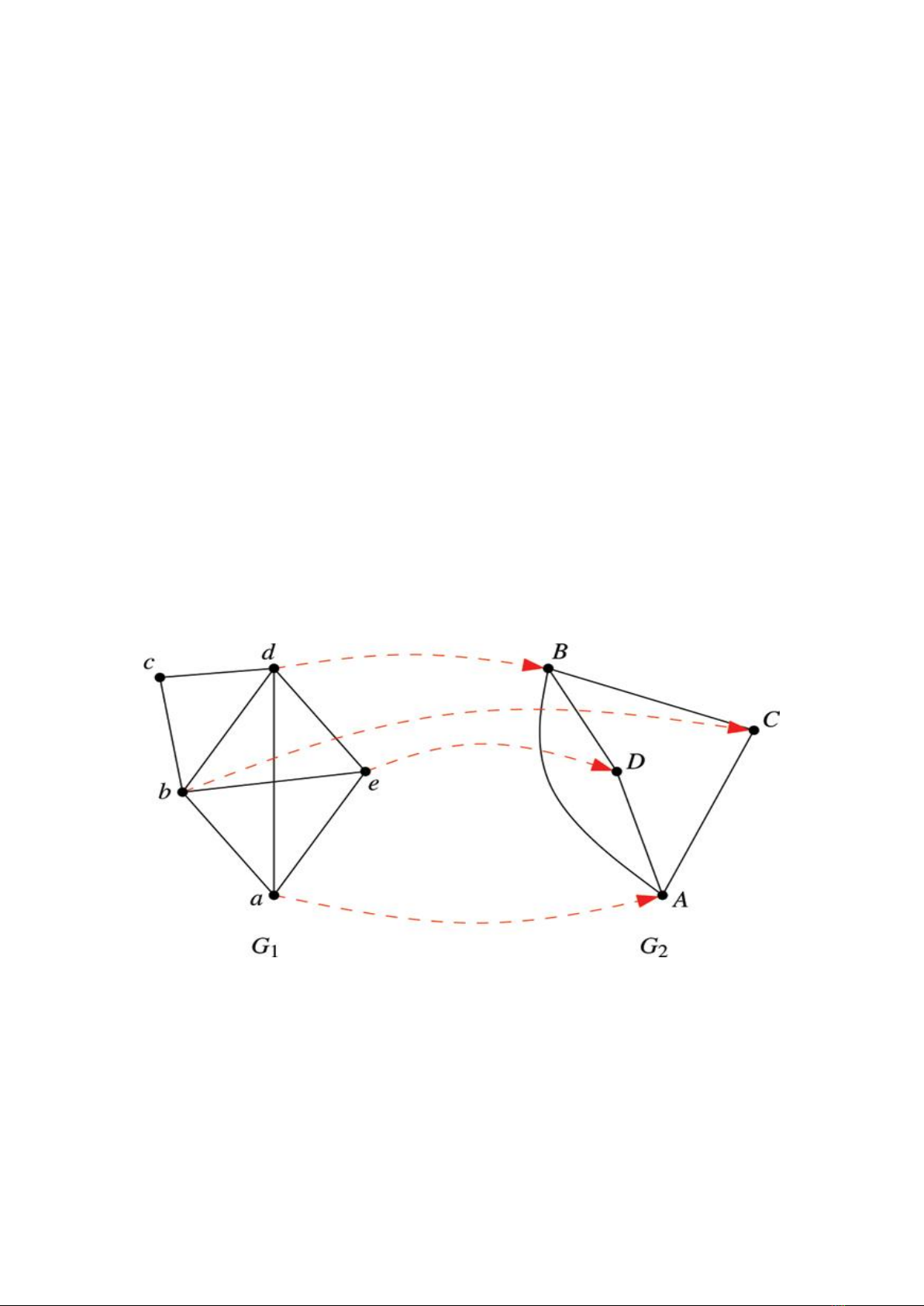
Let 𝐺1 = (𝑉1,𝐸1) and 𝐺2 = (𝑉2,𝐸2) be
PPI networks where 𝑉1, 𝑉2 denotes the sets of
nodes corresponding to the proteins. 𝐸1, 𝐸2
denotes the sets of edges corresponding to the
interactions between proteins. An alignment
network 𝐴12= (𝑉12, 𝐸12), in which each node in
𝑉12 can be presented as a pair <𝑢𝑖,𝑣𝑗>
where 𝑢𝑖∈𝑉1, 𝑣𝑗∈𝑉2. Every two nodes <
𝑢𝑖,𝑣𝑗> and <𝑢′𝑖,𝑣′𝑗> in 𝑉12 are distinct in
case of 𝑢𝑖 ≠ 𝑢′𝑖 and 𝑣𝑗 ≠ 𝑣′𝑗. The edge set of
alignment network are the so-called conserved
edge, that is, for edge between two nodes <
𝑢𝑖,𝑣𝑗> and <𝑢′𝑖,𝑣′𝑗> if and only if <
𝑢𝑖,𝑢′𝑖> ∈ 𝐸1 and <𝑣𝑗,𝑣′𝑗> ∈ 𝐸2.
Figure 1. An example of an alignment of two networks [17].
Although an official definition of successful
alignment network is not proposed, informally
the common goal of recent approaches is to
provide an alignment so that the edge set 𝐸12 is
large and each pair of node mappings in the set
𝑉12 contains proteins with high sequence
similarity [4, 18, 13, 14]. Formally, the
definition of pairwise global PPI network
alignment problem of 𝐴12 = (𝑉12, 𝐸12) is to
maximize the global network alignment score,
defined as follows [12]:

V.T.N. Anh et al. / VNU Journal of Science: Comp. Science & Com. Eng., Vol. 35, No. 1 (2019) 46-55
48
𝐺𝑁𝐴𝑆(𝐴12)= 𝛼 ×|𝐸12|+(1 − 𝛼)
× ∑ 𝑠𝑒𝑞(𝑢𝑖,𝑣𝑗)
∀ <𝑢𝑖,𝑣𝑗>
The constant 𝛼∈[0,1] in this equation is a
balancing parameter intended to vary the relative
importance of the network-topological similarity
(conserved edges) and the sequence similarities
reflected in the second term of sum. Each
𝑠𝑒𝑞(𝑢𝑖,𝑣𝑗) can be an approximately defined
sequence similarity score based on measures such
as BLAST bit-scores or E-values.
3. Related state-of-the-art work
By far there have been various
computational models proposed for global
alignment of PPI networks (e.g. [4, 12, 13, 14,
15, 16], as alluded in the introduction section).
Among them, to the best of our knowledge,
Spinal and FastAN are recently state-of-the-art.
3.1. SPINAL
SPINAL, proposed by Ahmet E. Aladağ
[12], is a polynomial runtime heuristic
algorithm, consisting of two phases: Coarse-
grained phase alignment phase and fine-grained
alignment phase. The first phase constructs all
pairwise initial similarity scores based on
pairwise local neighborhood matching. Using
the given similarity scores, the second phase
builds one-to-one mapping bfy iteratively
growing a local improvement subset. Both
phases make use of the construction of
neighborhood bipartite graphs and the
contributors as a common primitive. SPINAL is
tested on PPI networks of yeast, fly, human and
worm, demonstrating that SPINAL yields better
results than IsoRank of Singh et al. (2008) [13]
in terms of common objectives and runtime.
3.2. FastAN
FastAN, proposed by Dong et al. (2016)
[16], includes two phases, called Build and
Rebuild. They both employ the same strategy
similar to neighborhood search algorithms (see
Section 4.1) that repeatedly destroy and repair
the current found solution. The first phase is to
build an initial global alignment solution by
selecting iteratively an unaligned node from one
network, which has the most connections to
aligned nodes in the network, to pair with the
best-matched node from the other network (See
the Build phase, the first For loop, in Algorithm
1). The second phase follows the worst removal
strategy to destroy the worst parts (99%) of the
current solution based on their scores
independently calculated. FastAN keeps 1%
best pairs remained as a seeding set for
reconstructing the solution. The reconstructing
procedure is the same as the first phase. It
reconstructs the destroyed solution by
repeatedly adding best parts at the moment.
FastAN accept every newly created solution
from which it randomly choose one to follow.
Using the same objective function and the
dataset as SPINAL, FastAN yields much better
result than SPINAL [12].
4. Materials
4.1. Neighborhood search
Given 𝑆 the set of feasible solutions for
globally aligning two networks and I being an
instance (or input dataset) for the problem, we
denote 𝑆(𝐼) when we need to emphasise the
connection between the instance and solution
set. Function 𝑐: 𝑆 → ℝ maps from a solution to
its cost. 𝑆 is assumed to be finite, but is usually
an extremely large set. We assume that the
combinatorial optimization problem is a
maximization problem, that is, we want to find
a solution 𝑠∗ such that 𝑐(𝑠∗) >=𝑐(𝑠) ∀𝑠 ∈ 𝑆.
We define a neighborhood of a solution 𝑠 ∈
𝑆 as 𝑁(𝑠)⊆𝑆. That is, 𝑁 is a function that
maps a solution to a set of solutions. A solution
s is considered as locally optimal or a local
optimum with respect to a neighborhood 𝑁 if
𝑐(𝑠) >= 𝑐(𝑠’) ∀𝑠’ ∈ 𝑁(𝑠). With these
definitions it is possible to define a
neighborhood search algorithm. The algorithm
takes an initial solution 𝑠 as input. Then, it
computes 𝑠’ = 𝑎𝑟𝑔 𝑚𝑎𝑥𝑠′′∈𝑁(𝑠) {𝑐(𝑠′′)}, that

V.T.N. Anh et al. / VNU Journal of Science: Comp. Science & Com. Eng., Vol. 35, No. 1 (2019) 46-55
49
is, it searches the best solution 𝑠’ in the
neighborhood of s. If c(s’) > c(s) is found, the
algorithm performs an update 𝑠 = 𝑠’. The
neighborhood of the new solution s is
continuously searched until it is converged in a
region where local optimum 𝑠 is reached. The
local search algorithm stops when no improved
solution is found (see Algorithm 1). This
neighborhood search (NS), which always
accepts a better solution to be expanded, is
denoted a steepest descent (Pisinger) [19].
Algorithm 1. Neighborhood search in pseudo codes
𝑰𝑵𝑷𝑼𝑻: 𝑝𝑟𝑜𝑏𝑙𝑒𝑚 𝑖𝑛𝑠𝑡𝑎𝑛𝑐𝑒 𝐼
𝐶𝑟𝑒𝑎𝑡𝑒 𝑖𝑛𝑖𝑡𝑖𝑎𝑙 𝑠𝑜𝑙𝑢𝑡𝑖𝑜𝑛 𝑠𝑚𝑖𝑛 ∈𝑆(𝐼);
𝑾𝑯𝑰𝑳𝑬 (𝑠𝑡𝑜𝑝𝑝𝑖𝑛𝑔 𝑐𝑟𝑖𝑡𝑒𝑟𝑖𝑎 𝑛𝑜𝑡 𝑚𝑒𝑡) {
𝑠′= 𝑟(𝑑(𝑠));
𝑰𝑭 𝑎𝑐𝑐𝑒𝑝𝑡(𝑠,𝑠′) {
𝑠 = 𝑠’;
𝑰𝑭 𝑐(𝑠′)> 𝑐(𝑠𝑚𝑖𝑛)
𝑠𝑚𝑖𝑛 =𝑠′;
}
}
𝒓𝒆𝒕𝒖𝒓𝒏 𝑠𝑚𝑖𝑛
4.2. Large neighborhood search
Large neighborhood search (LNS) was
originally introduced by Shaw [20]. It is a meta-
heuristic that neighborhood is defined implicitly
by a destroy-and-repair function. A destroy
function destructs part of the current solution 𝑠
while repair function rebuilds the destroyed
solution. The destroy function should pre-
define a parameter, which controls the degree of
destruction. The neighborhood 𝑁(𝑠) of a
solution 𝑠 is calculated by applying the destroy-
and-repair function.
4.3. Adaptive Large Neighborhood search
Adaptive Large Neighborhood Search
(ALNS) is an extension of Large Neighborhood
Search and was proposed by Ropke and
Prisinger [19]. Naturally, different instances of
an optimization problem are handled by
different destroy and repair functions with
varying level of success. It may difficult to
decide which heuristics are used to yield the
best result in each instance. Therefore, ALNS
enables user to select as many heuristics as he
wants. The algorithm firstly assigns for each
heuristic a weight which reflects the probability
of success. The idea, that passing success is
also a future success, is applied. During the
runtime, these weights are adjusted periodically
every 𝑃𝑢 iterations. The selection of heuristics
based on its weights. Let 𝐷 = {𝑑𝑖 |𝑖=1..𝑘}
and 𝑅 = {𝑟𝑖 |𝑖=1..𝑙} are sets of destroy
heuristics and repair heuristics. The weights of
heuristics are 𝑤(𝑟𝑖) and 𝑤(𝑑𝑖). 𝑤(𝑟𝑖) and
𝑤(𝑑𝑖) are initially set as 1, so the probability of
selection of heuristics are:
𝑝(𝑟𝑖)= 𝑤(𝑟𝑖)
∑𝑤(𝑟𝑗)
𝑙
𝑗=1 and 𝑝(𝑑𝑖)= 𝑤(𝑑𝑖)
∑𝑤(𝑑𝑗)
𝑘
𝑗=1
Apart from the choice of the destroy-and-
repair heuristics and weight adjustment every
update period, the basic structure of ALNS is
similar LNS (see Algorithm 2).
Algorithm 2: Adaptive Large Neighborhood
Search algorithm
𝑰𝑵𝑷𝑼𝑻: 𝑝𝑟𝑜𝑏𝑙𝑒𝑚 𝑖𝑛𝑠𝑡𝑎𝑛𝑐𝑒 𝐼
𝐶𝑟𝑒𝑎𝑡𝑒 𝑖𝑛𝑖𝑡𝑖𝑎𝑙 𝑠𝑜𝑙𝑢𝑡𝑖𝑜𝑛 𝑠𝑚𝑖𝑛 ∈𝑆(𝐼);
𝑾𝑯𝑰𝑳𝑬 (𝑠𝑡𝑜𝑝𝑝𝑖𝑛𝑔 𝑐𝑟𝑖𝑡𝑒𝑟𝑖𝑎 𝑛𝑜𝑡 𝑚𝑒𝑡) {
FOR i = 1 TO 𝑝𝑢 DO {
select 𝑟 ∈ 𝑅,𝑑 ∈ 𝐷 according to
probability;
𝑠′= 𝑟(𝑑(𝑠));
𝑰𝑭 𝑎𝑐𝑐𝑒𝑝𝑡(𝑠,𝑠′) {
𝑠 = 𝑠’;
𝑰𝑭 𝑐(𝑠′)> 𝑐(𝑠𝑚𝑖𝑛)
𝑠𝑚𝑖𝑛 =𝑠′;
}
update weight 𝑤, and probability 𝑝;
}𝒓𝒆𝒕𝒖𝒓𝒏 𝑠𝑚𝑖𝑛
5. Proposed model
We note that FastAN still has some
limitations, including: (i) randomly choosing a

V.T.N. Anh et al. / VNU Journal of Science: Comp. Science & Com. Eng., Vol. 35, No. 1 (2019) 46-55
50
newly constructed solution to follow may yield
the unexpected results, gearing to the local
optimum by chance. (ii) The fixed degree of
destruction at 99% may reduce the flexibility of
neighborhood searching process. Setting this
degree too large can be used to diverse the
search space, however, would cause the best
results hardly to be reached. Newly constructed
solutions are not real neighbors of the current
solution, thus being totally irrelevant solutions).
(iii) The heuristic worst part removal of the
current solution may get FastAN stuck in a
local optimum because of the absence of
diversity. Moreover, using only one heuristic
does not guarantee the best result found for
different instances of problem. (iv) The basic
greedy heuristic in ALNS is employed to repair
destroyed solutions. Although it always
guarantees better solutions to be yielded, but it
is not the optimal way to construct the best
solution. There is another better heuristic called
n-regret could be employed. (v) Using only one
destroy heuristic and one repair (construction)
heuristic does not provide the weight
adjustment. Two heuristics are always chosen
with 100% of probability.
To this end, in this paper, we aim at
eliminating those limitations by proposing a
novel global protein-protein network alignment
model that is mainly based on FastAN. Unlike
FastAN, which employs a neighborhood search
algorithm, the proposed model improves
FastAN by adopting a rigorous adaptive large
neighborhood search (ALNS) strategy for the
second phase (namely Rebuild) of FastAN. The
Build phase is similar to that of FastAN (See
Alogrithm 3).
Alogrithm 3: Pseudo code for our proposed PPI
alignment algorithm
𝑰𝑵𝑷𝑼𝑻: 𝐺1=(𝑉1,𝐸1), 𝐺2=(𝑉2,𝐸2),
Similarity Score Seq[i][j], balance factor α
𝑶𝑼𝑻𝑷𝑼𝑻: An alignment 𝐴12
//Build Phase, similar to that of FastAN [21]
𝑉12 = <𝑖,𝑗> //with seq[i][j] is maximum
𝑭𝑶𝑹 𝑘=2 𝑻𝑶 | 𝑉1| 𝑫𝑶 {
𝑖=𝑓𝑖𝑛𝑑_𝑛𝑒𝑥𝑡_𝑛𝑜𝑑𝑒(𝐺1);
𝑗=𝑓𝑖𝑛𝑑_𝑏𝑒𝑠𝑡_𝑚𝑎𝑡𝑐ℎ(𝑖,𝐺1,𝐺2);
𝑉12 = 𝑉12 ∩ <𝑖,𝑗>;
}
//Rebuild phase
𝑭𝑶𝑹 𝑖𝑡𝑒𝑟 = 1 𝑻𝑶 𝑛_𝑖𝑡𝑒𝑟 𝑫𝑶 {
𝑑 = 𝑔𝑒𝑡_𝑑(𝑑𝑚𝑖𝑛,𝑑𝑚𝑎𝑥);
de𝑡𝑟𝑜𝑦_ℎ𝑒𝑢𝑟𝑖𝑠𝑡𝑖𝑐 =
𝑠𝑒𝑙𝑒𝑐𝑡_𝑑𝑒𝑠𝑡𝑟𝑜𝑦_ℎ𝑒𝑢𝑟𝑖𝑠𝑡𝑖𝑐();
𝑟𝑒𝑝𝑎𝑖𝑟_ℎ𝑒𝑢𝑟𝑖𝑠𝑡𝑖𝑐 =
𝑠𝑒𝑙𝑒𝑐𝑡_𝑟𝑒𝑝𝑎𝑖𝑟_ℎ𝑒𝑢𝑟𝑖𝑠𝑡𝑖𝑐();
𝑛𝑒𝑤_𝑠𝑜𝑙=
𝑑𝑒𝑠𝑡𝑟𝑜𝑦(𝑑𝑒𝑠𝑡𝑟𝑜𝑦_ℎ𝑒𝑢𝑟𝑖𝑠𝑡𝑖𝑐,𝑉12,𝑑);
𝑛𝑒𝑤_𝑠𝑜𝑙=
𝑟𝑒𝑝𝑎𝑖𝑟(𝑟𝑒𝑝𝑎𝑖𝑟_ℎ𝑒𝑢𝑟𝑖𝑠𝑡𝑖𝑐,𝑛𝑒𝑤_𝑠𝑜𝑙);
//reward for successful heuristics
𝑰𝑭 (𝐺_𝐵𝐸𝑆𝑇 < 𝑠𝑐𝑜𝑟𝑒(𝑛𝑒𝑤_𝑠𝑜𝑙)) {
𝐺_𝐵𝐸𝑆𝑇 = 𝑠𝑐𝑜𝑟𝑒(𝑛𝑒𝑤_𝑠𝑜𝑙);
𝑟𝑒𝑤𝑎𝑟𝑑(𝑑𝑒𝑠𝑡𝑟𝑜𝑦_ℎ𝑒𝑢𝑟𝑖𝑠𝑡𝑖𝑐,𝑟𝑒𝑝𝑎𝑖𝑟_ℎ𝑒𝑢𝑟𝑖𝑠𝑡𝑖𝑐,𝛿1);
}
𝑰𝑭 (𝑠𝑐𝑜𝑟𝑒(𝑉12) < 𝑠𝑐𝑜𝑟𝑒(𝑛𝑒𝑤_𝑠𝑜𝑙))
𝑟𝑒𝑤𝑎𝑟𝑑(𝑑𝑒𝑠𝑡𝑟𝑜𝑦_ℎ𝑒𝑢𝑟𝑖𝑠𝑡𝑖𝑐,𝑟𝑒𝑝𝑎𝑖𝑟_ℎ𝑒𝑢𝑟𝑖𝑠𝑡𝑖𝑐,𝛿2);
𝑰𝑭 (𝑎𝑐𝑐𝑒𝑝𝑡(𝑉12,𝑛𝑒𝑤_𝑠𝑜𝑙)) {
𝑉12 =𝑛𝑒𝑤_𝑠𝑜𝑙;
𝑟𝑒𝑤𝑎𝑟𝑑(𝑑𝑒𝑠𝑡𝑟𝑜𝑦_ℎ𝑒𝑢𝑟𝑖𝑠𝑡𝑖𝑐,𝑟𝑒𝑝𝑎𝑖𝑟_ℎ𝑒𝑢𝑟𝑖𝑠𝑡𝑖𝑐,𝛿3);
}
𝑰𝑭 (𝑖𝑡𝑒𝑟 % 𝑢𝑝𝑑𝑎𝑡𝑒_𝑝𝑒𝑟𝑖𝑜𝑑 == 0)
weight_𝑎𝑑𝑗𝑢𝑠𝑡𝑚𝑒𝑛𝑡();
}
𝒓𝒆𝒕𝒖𝒓𝒏 𝑉12;
The proposed algorithm uses a simple
Threshold Acceptance (TA) heuristic for
adaptive large neighborhood search. TA accepts
any solutions of which its difference from the
best so far (G-BEST) is not greater than T, a
manually given parameter in range
[0, positive inf) (see Procedure 1).
Procedure 1. Accept function used for adaptive large
neighborhood search
Boolean accept_function (sol, new_sol) {
IF (𝑐𝑜𝑠𝑡𝑠𝑜𝑙 −𝑐𝑜𝑠𝑡𝑛𝑒𝑤_𝑠𝑜𝑙 ≤𝑇 )
𝒓𝒆𝒕𝒖𝒓𝒏 𝑇𝑟𝑢𝑒;
𝒓𝒆𝒕𝒖𝒓𝒏 𝐹𝑎𝑙𝑠𝑒;
}
Note that the threshold T is set as a constant
rather than increasing or decreasing due to the


![Tài liệu học phần Enzyme và protein [mới nhất]](https://cdn.tailieu.vn/images/document/thumbnail/2024/20240408/khanhchi090625/135x160/7441712572025.jpg)

![Tài liệu giảng dạy Sinh học đại cương [mới nhất]](https://cdn.tailieu.vn/images/document/thumbnail/2021/20210412/tradaviahe20/135x160/118910721.jpg)
![Tổng luận Sinh học tổng hợp: [Thông tin chi tiết/ Nghiên cứu mới nhất]](https://cdn.tailieu.vn/images/document/thumbnail/2021/20210107/trinhthamhodang1217/135x160/2611610008754.jpg)


%20--%3e%3cdefs%3e%3cstyle%3e%20.st0%20{%20fill:%20%23fff;%20}%20.st1%20{%20fill:%20%237800fa;%20}%20%3c/style%3e%3c/defs%3e%3cpath%20class='st1'%20d='M117.78,12.18H43.11c2.9,3.47,4.65,7.94,4.65,12.82,0,5.6-2.3,10.66-6.01,14.29h76.02l7.22-13.56-7.22-13.56Z'/%3e%3cg%3e%3cpath%20class='st0'%20d='M53.58,26.17h-.59v-1.46h.59v-4.96h2.83c1.78,0,2.67.94,2.67,2.82v5.76c0,1.87-.89,2.81-2.67,2.81h-2.83v-4.96ZM55.36,21.37v3.34h1.1v1.46h-1.1v3.34h1.01c.61,0,.91-.37.91-1.1v-5.93c0-.74-.3-1.1-.91-1.1h-1.01Z'/%3e%3cpath%20class='st0'%20d='M65.99,31.14h-1.8l-.31-2.07h-2.19l-.31,2.07h-1.64l1.82-11.39h2.62l1.82,11.39ZM65.28,18.04c-.25.46-.51.77-.75.94-.21.15-.47.22-.79.22-.26,0-.57-.07-.92-.22l-.38-.15c-.14-.05-.26-.07-.37-.07-.3,0-.53.18-.71.54l-.91-.68c.25-.46.51-.77.75-.94.21-.14.48-.21.79-.21.26,0,.57.07.92.21l.38.15c.14.05.26.07.37.07.3,0,.53-.18.71-.54l.91.68ZM61.91,27.52h1.73l-.87-5.76-.87,5.76Z'/%3e%3cpath%20class='st0'%20d='M74.53,26.89v1.52c0,1.91-.89,2.86-2.67,2.86s-2.67-.95-2.67-2.86v-5.93c0-1.91.89-2.86,2.67-2.86s2.67.95,2.67,2.86v1.11h-1.69v-1.22c0-.75-.31-1.12-.93-1.12s-.93.37-.93,1.12v6.15c0,.74.31,1.11.93,1.11s.93-.37.93-1.11v-1.63h1.69Z'/%3e%3cpath%20class='st0'%20d='M81.4,31.14h-1.8l-.31-2.07h-2.19l-.31,2.07h-1.64l1.82-11.39h2.62l1.82,11.39ZM75.9,19.2l1.52-1.91h1.71l1.51,1.91h-1.61l-.76-.95-.75.95h-1.61ZM77.32,27.52h1.73l-.87-5.76-.87,5.76ZM83.1,15.99l-1.76,1.91h-1.26l1.17-1.91h1.86Z'/%3e%3cpath%20class='st0'%20d='M84.86,19.75c1.78,0,2.67.94,2.67,2.82v1.48c0,1.87-.89,2.81-2.67,2.81h-.85v4.28h-1.79v-11.39h2.64ZM84.01,21.37v3.86h.85c.58,0,.87-.36.87-1.08v-1.71c0-.71-.29-1.07-.87-1.07h-.85Z'/%3e%3cpath%20class='st0'%20d='M93.51,19.75c1.78,0,2.67.94,2.67,2.82v1.48c0,1.87-.89,2.81-2.67,2.81h-.85v4.28h-1.79v-11.39h2.64ZM92.66,21.37v3.86h.85c.58,0,.87-.36.87-1.08v-1.71c0-.71-.29-1.07-.87-1.07h-.85Z'/%3e%3cpath%20class='st0'%20d='M98.8,31.14h-1.79v-11.39h1.79v4.88h2.03v-4.88h1.83v11.39h-1.83v-4.88h-2.03v4.88Z'/%3e%3cpath%20class='st0'%20d='M105.36,24.55h2.46v1.62h-2.46v3.34h3.09v1.63h-4.88v-11.39h4.88v1.63h-3.09v3.18ZM108.17,17.29l-1.76,1.91h-1.26l1.17-1.91h1.86Z'/%3e%3cpath%20class='st0'%20d='M112.2,19.75c1.78,0,2.67.94,2.67,2.82v1.48c0,1.87-.89,2.81-2.67,2.81h-.85v4.28h-1.79v-11.39h2.64ZM111.35,21.37v3.86h.85c.58,0,.87-.36.87-1.08v-1.71c0-.71-.29-1.07-.87-1.07h-.85Z'/%3e%3c/g%3e%3ccircle%20class='st1'%20cx='25'%20cy='25'%20r='20'/%3e%3cpath%20class='st0'%20d='M32.78,19.27c2.92,0,4.43,2.55,5.28,5.33l.71,2.17c.14.38-.33.75-.71.75h-5.61c.19-.33.24-.71.09-1.08l-.75-2.45c-.43-1.32-.99-2.64-1.79-3.77.75-.57,1.65-.94,2.78-.94h0ZM25,18.38c3.25,0,4.9,2.78,5.89,5.89l.76,2.45c.14.42-.33.8-.8.8h-11.69c-.42,0-.94-.38-.8-.8l.75-2.45c.99-3.11,2.64-5.89,5.89-5.89h0ZM25,11.35c1.74,0,3.11,1.37,3.11,3.11s-1.37,3.11-3.11,3.11-3.11-1.41-3.11-3.11,1.41-3.11,3.11-3.11h0ZM17.27,19.27c1.08,0,1.98.38,2.73.94-.8,1.13-1.37,2.45-1.74,3.77l-.8,2.45c-.14.38-.05.75.09,1.08h-5.56c-.42,0-.9-.38-.75-.75l.71-2.17c.9-2.78,2.41-5.33,5.33-5.33h0ZM17.27,12.91c1.51,0,2.78,1.27,2.78,2.83s-1.27,2.83-2.78,2.83-2.83-1.27-2.83-2.83,1.27-2.83,2.83-2.83h0ZM32.78,12.91c1.56,0,2.78,1.27,2.78,2.83s-1.23,2.83-2.78,2.83-2.83-1.27-2.83-2.83,1.27-2.83,2.83-2.83h0ZM27.07,28.56v.09c0,.57-.24,1.08-.61,1.46h0v.05c-.38.33-.9.57-1.46.57s-1.08-.24-1.46-.61h0c-.38-.38-.61-.9-.61-1.46v-.09h1.41v.09c0,.19.05.38.19.47v.05c.09.09.28.19.47.19s.38-.09.47-.19v-.05c.14-.09.24-.28.24-.47t-.05-.09h1.41ZM30.99,28.56v.09c0,1.65-.66,3.16-1.74,4.24-1.08,1.08-2.59,1.79-4.24,1.79s-3.16-.71-4.24-1.79l-.05-.05c-1.04-1.08-1.7-2.55-1.7-4.2v-.09h1.41v.09c0,1.27.47,2.4,1.27,3.25h.05c.85.85,1.98,1.37,3.25,1.37s2.4-.52,3.25-1.37c.85-.8,1.37-1.98,1.37-3.25v-.09h1.37ZM34.99,28.56v.09c0,2.78-1.13,5.28-2.92,7.07-1.79,1.79-4.29,2.92-7.07,2.92s-5.23-1.13-7.07-2.92c-1.79-1.79-2.92-4.29-2.92-7.07v-.09h1.41v.09c0,2.4.94,4.53,2.5,6.08,1.56,1.56,3.72,2.5,6.08,2.5s4.52-.94,6.08-2.5c1.56-1.56,2.5-3.68,2.5-6.08v-.09h1.41Z'/%3e%3c/svg%3e)