An open close multiple travelling salesman problem with single depot

Chia sẻ: Huỳnh Lê Khánh Thi | Ngày: | Loại File: PDF | Số trang:16

Thêm vào BST

Báo xấu

26
lượt xem 1
download

Download Vui lòng tải xuống để xem tài liệu đầy đủ

This paper introduces a novel practical variant, namely an open close multiple travelling salesmen problem with single depot (OCMTSP) that concerns the generalization of classical travelling salesman problem (TSP).

Chủ đề:

Bình luận(0) Đăng nhập để gửi bình luận!

Lưu

Nội dung Text: An open close multiple travelling salesman problem with single depot

Decision Science Letters 8 (2019) 121–136 Contents lists available at GrowingScience Decision Science Letters homepage: www.GrowingScience.com/dsl An open close multiple travelling salesman problem with single depot Jayanth Kumar Thenepallea and Purusotham Singamsettya* aVellore Institute of Technology, Vellore, India CHRONICLE ABSTRACT Article history: This paper introduces a novel practical variant, namely an open close multiple travelling Received January 16, 2018 salesmen problem with single depot (OCMTSP) that concerns the generalization of classical Received in revised format: travelling salesman problem (TSP). In OCMTSP, the overall salesmen can be categorized into July 10, 2018 internal/permanent and external/outsourcing ones, where all the salesmen are positioned at the Accepted August 8, 2018 Available online depot city. The primary objective of this problem is to design the optimal route such that all August 12, 2018 salesmen start from the depot/base city, and then visit a given set of cities. Each city is to be Keywords: visited precisely once by exactly one salesman, and only the internal salesmen have to return to Open close multiple travelling the depot city whereas the external ones need not return. To find optimal solutions, an exact salesmen problem pattern recognition technique based Lexi-search algorithm (LSA) is developed which has been Lexi-search algorithm subjected in Matlab. Comparative computational results of the LSA have been made with the Pattern recognition technique existing methods for general multiple travelling salesman problem (MTSP). Further, to test the performance of LSA, computational experiments have been carried out on some benchmark as well as randomly generated test instances for OCMTSP, and results are reported. The overall computational results demonstrate that the proposed LSA is efficient in providing optimal and sub-optimal solutions within the considerable CPU times. © 2018 by the authors; licensee Growing Science, Canada. 1. Introduction The classical travelling salesman problem (TSP) is one of the typical problems in combinatorial optimization and which is known to be NP-hard. It is the problem of determining an optimal closed Hamiltonian path in a given directed/undirected network. The multiple travelling salesmen problem (MTSP) is a generalized version of TSP, which is more complicated than the classical TSP (Berenguer, 1979; Carter & Ragsdale, 2006). This TSP consists of exactly one tour whereas the MTSP involves a set of m disjoint tours for m salesman. The MTSP with single depot can be formally defined as follows: Let a given set of n cities is to be traversed by m (n > m; m >1) salesmen, where all the salesmen are positioned at the depot city. The problem is to determine m tours such that all the salesmen have to start from the depot city, visits each city exactly once and return to the depot city with optimal traversal cost/distance. The various applications of MTSP emerge in real world problems such as printing press scheduling, school bus routing, crew scheduling, interview scheduling, hot rolling scheduling, mission planning and design of global navigation satellite system (GNSS) (Kara & Bektas, 2006; Bolanos et al., 2015; Kiraly et al., 2016). Due to its diversified applications, the MTSP has been extended to many practical variants such as MTSP with multiple depots, fixed number of salesmen, fixed charges, and * Corresponding author. Tel.: +919948536763 E-mail address: drpurusotham.or@gmail.com (P. Singamsetty) © 2019 by the authors; licensee Growing Science, Canada. doi: 10.5267/j.dsl.2018.8.002
122 time windows (Ali & Kennington, 1986; Lenstra & Kan, 1979; Kara & Bektas, 2006). Since, the MTSP is an exceptional variant of TSP, the solution procedures available for TSP can also be applicable for MTSP. Furthermore, the MTSP can be extended to various practical situations like distribution system in transportation, particularly in vehicle routing problems (VRP). This study keeps much attention on MTSP than the usual TSP. The solution methods used to solve MTSP can be categorized into heuristics, meta-heuristics, and exact approaches. Different heuristic algorithms have been presented in the literature to solve MTSP and its variants. The first heuristic algorithm for min-sum MTSP was appeared in (Russell, 1977), where it utilizes an extension of prominent Lin and Kernighan heuristic. A two phase heuristic algorithm has been proposed to solve no-depot min-max MTSP, where m tours are established in the first phase, and these tours are explored in phase two (Na, 2007). A neural network based solution procedure (Wacholder et al., 1989) has been developed for solving MTSP. A competition based neural network approach (Somhom et al., 1999) for MTSP with minmax objectives has been proposed. Soylu (2015) presented a general variable neighborhood search algorithm (VNS) for MTSP and which was then applied to a real life problem raised in traffic signalization network of Kayseri province in Turkey. The exact solution methods for different models of MTSP can be found in (Gavish & Srikanth, 1986; Franca, 1995; Bektas, 2006; Bhavani & Sundara Murthy, 2006; Sarin et al., 2014; Balkrishna & Murthy, 2012). Apart from the heuristics and exact algorithms, bio-inspired approaches like genetic and evolutionary algorithms have been developed to tackle MTSP and its variants in the literature. Yousefikhoshbakht et al. (2013) suggested a modified version of ant colony optimization (ACO), which exploits an efficient method to overcome the local optimum. A genetic algorithm based novel approach (Kiraly & Abonyi, 2010) has been developed to tackle MTSP. Larki and Yousefikhoshbakht (2014) proposed an efficient evolutionary optimization approach, which includes the composition of modified imperialist competitive algorithm and Lin-Kernigan heuristic. A new steady-state grouping genetic algorithm (GGA-SS) (Singh & Baghel, 2009) has been developed for MTSP. A genetic algorithm utilizing new crossover operator known to be two part chromosome crossover (TCX) (Yuan et al., 2013) has been suggested for solving MTSP. Sarin et al. (2014) studied the multiple asymmetric travelling salesmen problem with and without effect of precedence constraints. Venkatesh and Singh (2015) presented two meta-heuristics such as artificial bee colony (ABC) and invasive weed optimization (IWO) algorithms to tackle MTSP. Wang et al. (2015) developed an enhanced non-dominated sorting genetic algorithm II (NSGA-II) by utilizing the set of experience of knowledge structures (SOEKS) to tackle MTSP. Bolanos et al. (2016) developed an effective genetic algorithm (GA) to solve MTSP. Changdar et al. (2016) studied the solid MTSP in the fuzzy environment and proposed a hybrid algorithm based genetic and ant colony optimization approach. From the extensive literature review, it is observed that the most of the studies of MTSP and its variants dealt with the assumption that all the salesman need to return to the depot city after visiting the given cities. However, many real time scenarios can be seen that the salesmen may or may not to come back to the depot city. Outsourcing is one such scenario that becomes a widespread business strategy followed by any organization and serves increasing productivity in services and operations. Usually, outsourcing takes place in logistics transportation and distribution activities where the tasks are to be collaboratively done by permanent and temporary/outsourcing resources to cut down the overall expenses and enhance the productivity, service quality. Any organization may be experienced in raising the demand for services on particular time horizons. However, this exceptional demand does not support the investment for organizations in hiring new permanent sources. Thus, it is inevitable to collaborate with external sources to fulfil the additional requirements. With this motivation, in this paper, a novel practical variant of MTSP namely an open close multiple travelling salesmen problem with single depot (OCMTSP) is considered, where the open and closed paths are simultaneously concerned with the solution. Closed path refers that the salesman starts and finishes at the depot city, while open path refers the salesman need not come back to the depot city. Here, the open and closed paths are designed by the external and internal salesmen respectively, where the internal salesmen are referred to as organizational permanent sources and the external ones are called temporary/ outsourcing people hired by the organization. In the general MTSP, all the salesmen start and end their tours at the
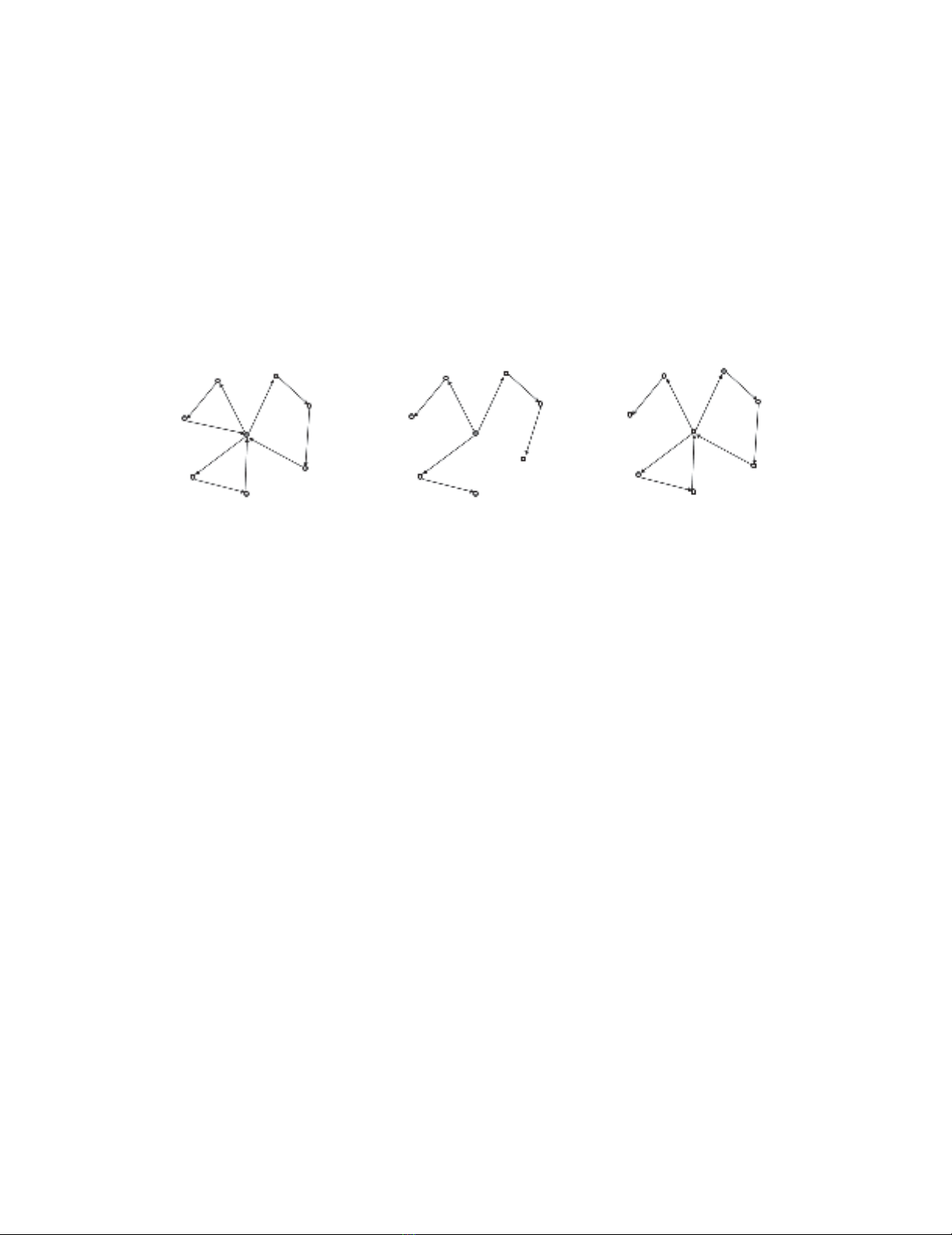
J. K. Thenepalle and P. Singamsetty / Decision Science Letters 8 (2019) 123 depot city, forms closed tours and is referred to as closed MTSP and conversely, if all the salesmen are restricted not to return to the depot city, the problem is called as open MTSP. The problem OCMTSP is a combination of both open and closed MTSP. For ease of understanding, Figure 1 depicts three heterogeneous variants of single depot MTSP with three salesmen. In Fig. 1 (a) represents the MTSP with closed paths, (b) illustrates the MTSP with open paths, and (c) shows the MTSP with mixed paths (combination of open and closed paths). In order to solve this OCMTSP optimally, an exact algorithm namely, the pattern recognition technique based Lexi-search algorithm (LSA) is developed. The problem OCMTSP has several real time applications in transportation and distribution system. The paper is arranged as follows: The subsequent section will formally define the proposed problem and a zero-one integer programming model. Section 3 describes the preliminaries connected to the solution procedure. The proposed Lexi-search algorithm (LSA) is presented in Section 4, whereas Section 5 provides a numerical illustration for OCMTSP. Computational details are reported in Section 6. Finally, concluding remarks are summarized in Section 7. (a) (b) (c) Fig. 1. Three heterogeneous variants of MTSP with a single depot' instead of 'Three distinct variants of MTSP with respect to single depot 2. Problem description and formulation This section is devoted to proposing formulation for OCMTSP. The OCMTSP can be formally defined as follows: Let G  ( N , E) be a directed connected graph, where N  {1, 2,..., n} be the given set of n cities/nodes (including depot city) and E be an edge/arc set. A non-negative asymmetric distance dij is associated with each edge (i, j )  E and indicates the travel distance from i th city to j th city. Let K  {1, 2,..., m} be the set of m (where m  p  q; m  n) salesman, among them p internal salesman and q external salesman are positioned at a depot/base city (say  ,   N ) . For each edge (i, j )  E , xij  1 , if and only if the salesman traverses from i th city to j th city, and xij  0 , otherwise. The cities other than the depot are known to be intervening cities. The prpblem OCMTSP determines p closed paths and q open paths for respective internal and external salesman, such that each intervening city is to be visited by exactly one salesman and the overall distance traversed by m salesman is minimized. The following assumptions are used to formulate the model OCMTSP.  There are number of cities to be visited by salesmen, of which internal and external salesmen, all are positioned at the depot city.  All the salesmen have to start from the depot city and only internal salesmen need to return to the depot city, whereas the external ones need not to return.  There are closed paths and open paths associated with the feasible solution.  The number of internal salesmen and external salesmen are predefined.  The number of cities to be assigned dynamically for internal and external salesmen such that the total travel distance is least.
124  Each city is to be visited exactly once by only one salesman except the depot city.  Each k th salesman visits a subset of cities dented by Sk , thus the number of cities visited by any salesman is bounded i.e. a salesman must visit at least 1 city and at most n  m  1 cities.  The entries in the distance matrix assume arbitrary units. Under these assumptions, the model OCMTSP is formulated as a zero-one integer programming problem as follows: n n Minimize Z = åå dij xij (1) i=1 j =1 Subject to the constraints n n åå i=1 j =1 xij = m + n - q -1 (2) n  x j 1 j  m,    N (3) n  x  p ,    N i 1 i (4) n x i 1 ij  1,  j  N / { } (5) n x j 1 ij  1,  i  N / { } (6) 1 £| S k | £ n - m + 1; " k Î K (7) +Sub tour/illegal tour elimination constraints (8) xij Î {0,1} " i, j Î N (9) In the above model, (1) represents the objective function that minimizes the overall distance traversed by m salesman. The constraint (2) ensures from the fact that any feasible solution consists of m  n  q  1 arcs. Constraints set (3-4) assures that m salesman depart from depot city and p salesman need to return the depot city  . Constraint sets (5-6) represents that a salesman enters into each city exactly once and exit from each city at most once. The constraint (7) imposes the lower and upper bound on the number of cities visited by any salesman so that no salesman is left ideal. The constraint (8) aims to eliminate the sub tours from the solution which are not feasible. Finally, the constraint (9) represents the binary variable i.e. xij  1 , if the edge (i, j )  E is traversed by a salesman and otherwise xij  0. 3. Preliminaries of LSA The main components associated to the Lexi-search algorithm (LSA) are described as follows: 3.1. Feasible solution A solution to the OCMTSP is said to be a feasible, if it satisfies all the problem constraints given in (2)-(9). 3.2.Pattern An indicator two-dimensional arrangement X which is connected to the solution is termed as pattern. A pattern X is said to be feasible pattern if the pattern X is feasible. The value of the pattern X is determined using (10), provides the overall travel distance and this is equal to the value of the objective function
J. K. Thenepalle and P. Singamsetty / Decision Science Letters 8 (2019) 125 n n (10) V ( X ) = å å d ij xij i=1 j =1 3.3. Alphabet table An alphabet table is formed by arranging the elements of the distance matrix D  [dij ] in non- decreasing order and indexed from 1 to n  n . Let SN  {1, 2,..., n } be the set of n  n ordered indices, 2 arrays d and Cd represent the distance and cumulative sums of the elements in D , respectively. Let the arrays R and C respectively denote row and column indices of the ordered elements in SN . The table comprises the set of ordered indices such as SN , d , Cd , R and C is referred as alphabet table. Let Lr  ( p1 , p2 , p3 ,..., pr ) be an ordered string of r indices from the set SN , where pi is a member of SN . The pattern Lr indicated by an ordered indices and these indices are independent of the order pi in the sequence. For uniqueness, the indices from SN are organized in non-decreasing order such that pi  pi 1 , i  1, 2,..., r 1. 3.4. Word and partial word An ordered sequence Lr  ( p1 , p2 , p3 ,..., pr ) is represented as a word of length r . A feasible word Lr is said to be a partial feasible word if r  m  n  q  1 and if r  m  n  q  1 , then it represents the full length feasible word or simply a word. Any one of the indices from SN can take up the prime position in the partial word Lr . A partial word Lr defines a block of words with Lr as a leader. If the block of word characterized by it has at least one feasible word then the leader is said to be feasible, otherwise infeasible. 3.5. Value of a word The value of the word Lr denoted by V (Lr ) is determined iteratively by using V ( Lr )  V (Lr 1)  d ( pr ) with V ( L0 )  0 , where d ( pr ) be the distance array which is organized in such a way that d ( pr )  d ( pr 1 ),  i  1, 2,..., n2  n . The value V ( Lr ) is similar to the value of V (X) . 3.6. Computation of bounds The effective setting of lower and upper bounds are more challenging to the class of NP-hard problems to control the search space. Initially, the upper bound of Lr is assumed to be a high value ( UB = VT = 9999) (for minimization objective functions) as a trial solution. The lower bound LB( Lr ) of the partial word Lr can be determined using the following formula: LB( Lr )  V ( Lr )  Cd ( pr  B  r )  Cd ( pr ), where B  n  p  1  m  n  q  1 . 4. Lexi-search algorithm Optimal solutions obtained by exact search methods have grown into more attractive in the context of solving combinatorial optimization problems in order to make effective decisions. The exact approaches can be observed as exhaustive and implicit search methods. One of the prominent implicit search technique is Branch and Bound method (B&B) (Little et al., 1963). LSA is one such implicit enumeration procedure, due to effective bound settings, only a fractional part of a solution space is investigated and converges to optimal solution systematically (Pandit, 1962), which was developed to tackle the loading problem. Infact, B&B can be seen as a special case of LSA. The LSA takes care of all the components of B&B such as the development of feasible solutions, feasibility checking and determining the bounds for the partial feasible solution. The entire search process is done in a precise manner and resembles to the search for an essence of a word in a dictionary, thus, the name is given as
126 “Lexi-search”. Moreover, this systematic search defends stack overflow and search time. The main difficulty of any problem utilizing implicit enumeration methods is (i) checking the feasibility (ii) setting effective bounds. There is a difficulty in testing the feasibility for few problems. To overcome this, a pattern recognition technique based Lexi-search approach (Murthy, 1976) has been developed and stated as follows: “A unique pattern is connected with each solution of a problem. Partial pattern represents a partial solution. An alphabet-table is characterizes with the assistance of which the words, representing the pattern are listed in a lexicographic or dictionary order. During the search for an optimal word, when a partial word is considered, first bounds are determined and then the partial words for which the value is less than the trail value are checked for the feasibility”. Proposed Lexi-search Algorithm The step by step procedure of Lexi-search algorithm is described as follows: Step 1: Initialization Initialize the distance matrix D  [dij ] , the required parameters m, n, p , q and UB = VT = 9999 (large value) and go to Step 2. Step 2: Construct an alphabet table using the given distance matrix D as discussed in the Section 3.3 and move to Step 3. Step 3: Bound Settings The algorithm starts with a partial word Lr  ( pr )  1, pr  SN , where the length of the partial word is unity, i.e. r 1. Determine the lower bound of a partial word LB(Lr ) as explained in Section 3.6. If LB( Lr )  VT , then go to Step 5, else go to Step 4. Step 4: If LB(Lr )  VT , then drop the partial word Lr and dismiss the block of words with Lr as leader. Since it does not yield an optimal solution and thus, reject all the partial words of the order r that succeeds Lr and go to Step 7. Step 5: Feasibility Checking If the partial word Lr satisfies the constraint set (2)-(9) then it is said to be feasible, otherwise, it is infeasible. If Lr is feasible, then accept it and continue for next partial word of order r 1 and go to Step 6, else proceed with the next partial word of order r by considering another letter that succeeds pr in its r th position and go to Step 3. Step 6: Concatenation If Lr is a full length feasible word of length r (i.e. r  m  n  q 1) , then replace VT by the value of LB( Lr ) and then go to Step 8. If Lr is a partial word, then it can be concatenated by using Lr 1  Lr *( pr 1 ) , where * indicates the concatenation operation and go to Step 3. Step 7: If all the words of order r are exhausted and length of the word Lr is 1, then the search mechanism is terminated and go to Step 9, else move to Step 8. Step 8: Backtracking Backtracking is adopted to explore the search space; the current VT is assumed as an upper bound and continues the search with next letter of the partial word of order r  1, go to Step 3. Repeat the Steps 3 to 8 until VT has no further improvement and ignore the feasible/infeasible solutions which are not constitute in the optimal solution. Go to Step 9. Step 9: Record the latest VT and the corresponding word Lr . Go to Step 10. Step 10: Stop
J. K. Thenepalle and P. Singamsetty / Decision Science Letters 8 (2019) 127 Finally, at the end of the search, VT provides the optimal solution and the word Lr give the position of the letters and one can find the optimal schedule for connectivity of given cities with the help of Lr . 5. Numerical Illustration A numerical example with 9 cities is considered to explain the concepts and the LSA for OCMTSP, for which N  {1, 2,3, 4,5, 6, 7,8,9} . The distance between each pair of cities assumes a non-negative quantity, can be asymmetric, represented as a distance matrix D and is given in Table 1, where ‘–’ indicates the disconnectivity or self-loop between the pair of cities. Let the depot city as  =1, assumed that there are three salesman ( m  3 ), in which two internal salesman ( p  2) and one external/outsourcing salesman (q  1) are positioned at the depot city. The problem is to find the best route plan for the three salesman to cover all the 9-cities such that the overall traversal distance is minimum. The asymmetric distance matrix D assumes the non-negative values (arbitrary units) and is given in Table 1. Table 1 Distance matrix (D) i\ j 1 2 3 4 5 6 7 8 9 1 - 10 15 95 66 55 29 2 21 2 61 - 55 22 50 72 1 58 29 3 45 50 - 69 7 89 22 78 59 4 91 67 75 - 35 27 34 89 63 5 60 36 90 31 - 50 61 77 12 6 3 82 20 70 39 - 77 28 5 7 16 57 26 86 53 19 - 69 46 8 13 14 54 8 84 37 87 - 42 9 17 32 68 30 48 79 52 44 - 5.1. Alphabet table Table 2 concerns the construction of alphabet table as discussed in Section 3.3 for the distance matrix D . The first three columns report that the serial number ( SN ) , distance (d ) and cumulative distance (Cd ) , respectively. The subsequent two columns provide the details about row ( R) and column (C ) indices, respectively. For convenience, a partial alphabet table is considered and given in Table 2. Table 2 Alphabet Table SN d Cd R C SN d Cd R C 1 1 1 2 7 16 21 183 1 9 2 2 3 1 8 17 22 205 3 7 3 3 6 6 1 18 22 227 2 4 4 5 11 6 9 19 26 253 7 3 5 7 18 3 5 20 27 280 4 6 6 8 26 8 4 21 28 308 6 8 7 10 36 1 2 22 29 337 1 7 8 12 48 5 9 23 29 366 2 9 9 13 61 8 1 24 30 396 9 4 10 14 75 8 2 25 31 427 5 4 11 15 90 1 3 – – – – – 12 16 106 7 1 72 95 3363 1 4 13 17 123 9 1 73 – – 1 1 14 19 142 7 6 – – – – – 15 20 162 6 3 81 – – 9 9 The first three columns report that the serial number . , distance and cumulative distance respectively. The subsequent two columns provide the details about row and column indices respectively. For convenience, a partial alphabet table is considered and given in Table 2.
128 5.2.Search table The logical flow of the developed LSA (presented in Section 4) is given through a numerical example in Table 3. Table 3 Search Table S.N 1 2 3 4 5 6 7 8 9 10 V LB R C Rem 1 1 1 75 2 7 A 2 2 3 75 1 8 A 3 3 6 75 6 1 A 4 4 11 75 6 9 R 5 5 13 85 3 5 A 6 6 21 85 8 4 A 7 7 31 85 1 2 A 8 8 43 85 5 9 A 9 9 56 85 8 1 R 10 10 57 88 8 2 R 11 11 58 91 1 3 A 12 12 74 91 7 1 A 13 13 91 91 9 1 R 14 14 93 93 7 6 R 15 15 94 94 6 3 R 16 16 95 95 1 9 R 17 17 96 96 3 7 R 18 18 96 96 2 4 R 19 19 100 100 7 3 R 20 20 101 101 4 6 A,VT=101 21 13 75 94 9 1 A 22 14 94 94 7 6 A,VT=94 23 14 77 97 7 6 >VT, R 24 12 59 95 7 1 >VT, R 25 9 44 89 8 1 R 26 10 45 93 8 2 R 27 11 46 98 1 3 >VT, R 28 8 33 91 5 9 A 29 9 46 91 8 1 R 30 10 47 95 8 2 >VT, R 31 9 34 96 8 1 >VT, R 32 7 23 93 1 2 A 33 8 35 93 5 9 A 34 9 48 93 8 1 A 35 10 62 93 8 2 R 36 11 63 96 1 3 >VT, R 37 10 49 97 8 2 >VT, R 38 9 36 98 8 1 >VT, R 39 8 25 100 5 9 >VT, R 40 6 14 94 8 4 >VT, R 41 4 8 87 6 9 A 42 5 15 87 3 5 A 43 6 23 87 8 4 A 44 7 33 87 1 2 A 45 8 45 87 5 9 R 46 9 46 91 8 1 R 47 10 47 95 8 2 >VT, R 48 8 35 93 5 9 R 49 9 36 98 8 1 >VT, R 50 7 25 95 1 2 >VT, R 51 6 16 96 8 4 >VT, R 52 5 10 98 3 5 >VT, R 53 3 4 88 6 1 A 54 4 9 88 6 9 R 55 5 11 99 3 5 >VT, R 56 4 6 101 6 9 >VT, R 57 2 2 89 1 8 A 58 3 5 89 6 1 A 59 4 9 89 6 9 R 60 5 12 100 3 5 >VT, R 61 4 7 102 6 9 >VT, R 62 2 3 103 6 1 >VT, R
J. K. Thenepalle and P. Singamsetty / Decision Science Letters 8 (2019) 129 Table 3 explains the details that how the algorithm enumerates the solutions as well as converges to the optimal solution. The column indexed by SN represents the serial number. Since n  9, m  3, p  2 and q  1 , therefore the total number of arcs required for the optimal schedule of OCMTSP is m  n  q  1  10 . Thus, the length of optimal feasible word becomes 10. The columns 1, 2, 3, 4, …, 10 of Table 3 represents the respective positions of the letters of a word Lr . The subsequent columns labelled as V , LB, R and C respectively represent the value, lower bound, row and column indices of the partial word. Finally, the column indexed by Rem represents the remarks of a partial word i.e. if a partial word is feasible then it is accepted and denoted by ‘A’, otherwise rejected and indicated by ‘R’. Here, serial number SN indicates the iteration count. 5.3.Optimal and sub-optimal solutions The set of solutions, which are observed from the search table are given in Table 4. Table 4 reports the details of feasible patterns, corresponding schedules, feasible (sub-optimal) and optimal solutions. The initial found pattern L10  {1, 2,3,5,6,7,8,11,12, 20} gives the objective function value VT  101 units that is noticed at 20th row of the Table 3. In order to improve this solution backtracking is performed. After performing the backtracking by considering the initial found solution (i.e. 101 units) as current upper bound, the best objective function value as VT  94 units and whose feasible pattern L10  {1, 2,3,5,6,7,8,11,13,14} is found at 22nd row of the Table 3. Table 3 clearly shows that the objective function value VT  94 units dominates all the other solutions, and hence the current solution (i.e. VT  94 units) become the optimal solution. This clearly shows the developed LSA is capable to enumerate the possible solutions that assist the decision maker to construct viable decisions with preferred solutions also. The graphical representation of respective feasible and optimal solutions is given in Fig. 2 and Fig. 3. Table 4 Optimal and Sub-optimal Solutions S.N Feasible Pattern Corresponding schedule Solution 1 , , , , , , , , , (2, 7), (1, 8), (6, 1), (3, 5), 101 (8, 4),(1, 2), (5, 9), (1, 3), (Sub-optimal) (7, 1), (4, 6) 2 , , , , , , , , , (2, 7), (1, 8), (6, 1), (3, 5), 94 (8, 4), (1, 2), (5, 9), (1, 3), (Optimal) (9, 1), (7, 6) Fig. 2. Feasible solution of OCMTSP Fig.3. Optimal solution of OCMTSP
130 6. Computational analysis This section presents the computational details of the proposed LSA over benchmark instances. In order to assess the LSA performance, first we compare our results with the existing results. We then, considered few standard instances from TSPLIB (Reinhelt, 2014) and evaluated the performance of LSA for OCMTSP. Finally, we extend our computational experiments to random instances to assess the performance of LSA. All the experiments were conducted by implementing the LSA in Matlab 2017a and then running on PC with 2.0 GHz, Intel(R) core i3 processor, 4 GB of RAM running Microsoft Windows 10 Operating System. 6.1. Comparative results of LSA with existing results To measure the solution quality, the results over the benchmark instances of proposed LSA was compared to the results of CPLEX, Benders and GA based ant colony optimization (ACO) methods reported in (Changdar et al., 2016). The comparative analysis is carried out on four asymmetric benchmark instances namely br17, ftv33, ftv35, and ftv38 taken from the TSPLIB and overall results about 12 cases are summarized in Table 5. From the results given in Table 5, the following remarks are noticed: a. The best found solutions for four cases namely br17 (with 2, 3 and 4 salesman) and ftv33 (with 2 salesman) using LSA coincides with the existing CPLEX, Benders, and GA based ACO approaches. b. For ftv33 (with 3 salesman) and ftv35 (with 2 salesman), the results of LSA coincides with CPLEX, Benders methods and better than the GA based ACO approach, while for ftv35 (with 3 salesman) and ftv38 (with 2 and 3 salesman), LSA results identical with Benders and GA based ACO methods and better than CPLEX method. c. For ftv35 (with 4 salesman) and ftv38 (with 4 salesman), LSA results matches with GA based ACO method and better than the Benders method, while for the same cases the blank results indicate that the results are not provided in the former works. d. Clearly it is seen that LSA is superior than CPLEX and Benders method in providing the optimal solution, while except the case ftv33 (with 4 salesman) GA based ACO provided the better solution than LSA, but the solution obtained by LSA for the same case is same as that of CPLEX and Benders method. e. From the overall results, the LSA is better than the CPLEX, Benders method and is competitive with GA based ACO method. Moreover, to visually evaluate the capability of the proposed LSA with CPLEX, Benders and GA methods on four standard test instances, the bar charts are presented. Figures 4, 5, 6 and 7 represents the four bar charts to compare the travel distance over the distinct number of salesman on the benchmark instances br17, ftv33, ftv35, and ftv38, respectively. In Fig. 4, it is seen that all the four methods are providing the same solutions on the benchmark instance br17 with 2, 3, and 4 salesman. In Fig. 5, it is observed that the proposed LSA results matches with CPLEX and Benders methods on the ftv33 with 2, 3, and 4 salesman, while the GA based ACO result on ftv33 with 4 salesman better than LSA. Similarly, in Fig. 6, it is witnessed that the proposed LSA results matches with CPLEX and Benders methods on the ftv35 with 2 salesman and far better than GA based ACO method. The LSA results matches with Benders and GA based ACO methods on the ftv35 with3 salesman. Finally, in Fig. 7, it is evident that the proposed LSA results matches with Benders and GA based ACO methods on ftv38 with 2 and 3 salesman and far better than CPLEX method.From the figures, it is seen that in most of the cases LSA works better than CPLEX, Benders method and is competitive with GA based ACO method.
J. K. Thenepalle and P. Singamsetty / Decision Science Letters 8 (2019) 131 6.2. Analyzing the performance of LSA for OCMTSP over benchmark and random instances In order to measure the performance of LSA for OCMTSP, four benchmark test instances namely br17, ftv33, ftv35, and ftv38 are taken from TSPLIB. The experiments were performed on each test instance by setting distinct values on the parameters namely, number of salesman (m) , number of internal salesman ( p) and number of external salesman (q) . Overall, 17 cases have been tested for four test instances and the results are reported in Table 6. Table 6 summarizes the best-found solutions using LSA for each case of the test instance within the predefined time limit of 3600 seconds. The route plans of the salesman with respect to the best solution of OCMTSP is given in Table 7. Table 5 Comparative results of LSA for MTSP using various existing algorithms (Changdar et al., 2016) Instance Number of CPLEX Benders GA based Proposed Salesmen Method ACO LSA 2 39 39 39 39 br17 3 42 42 42 42 4 47 47 47 47 2 1302 1302 1302 1302 ftv33 3 1328 1328 1342 1328 4 1367 1367 1352 1367 2 1489 1489 1511 1489 ftv35 3 1541 1511 1511 1511 4 − 1551 1532 1532 2 1551 1505 1505 1505 ftv38 3 1567 1521 1521 1521 4 − 1546 1532 1532 Table 8 provides a summary of the descriptive statistical results of CPU execution times of LSA for OCMTSP tested on randomly generated test instances ranging from 10 to 80 cities. The arc distance dij takes the random values over the range [1 300]. For each problem size, a set of 10 independent test instances are generated, together becomes 80 random instances and tested with distinct combinations of m , p and q . The columns Min., Max., Avg., and SD are the minimum, maximum, average CPU runtimes required to find the best solutions in all of the 10 runs and the standard deviation of the CPU runtimes, respectively.From the results reported in Table 8, it is observed that the average CPU runtimes required to solve the problems are ranging from 0.0688 seconds to 204.3234 seconds. However, the runtimes are little higher, but are practicably acceptable. It is seen that, the average CPU runtimes start increasing when the problems of size 30 or higher with different combinations of m , p and q . From overall results, an interesting observation is that apart from the problem size (n) , the combination of key parameters m , p , and q also decides the problem complexity and yet, solving larger instances may take higher CPU runtimes. Furthermore, for each of the data set, standard deviation (SD) is also measured and it is evident that the SD results are closer to zero. This shows that LSA CPU runtimes are less spread out from the average CPU runtimes. Fig. 4. Comparison of travel distance for br17 by Fig. 5. Comparison of travel distance for ftv33 by considering two, three and four salesmen considering two, three and four salesmen
132 Fig. 6. Comparison of travel distance for ftv35 by Fig. 7. Comparison of travel distance for ftv38 by considering two and three salesmen considering two, and three salesmen Table 6 Results of LSA for OCMTSP on benchmark instances Instance |N| m p q Best solution br17 17 5 3 2 35 6 4 2 41 4 3 1 35 5 2 3 30 6 2 4 33 ftv33 33 5 3 2 1240 7 4 3 1278 6 3 3 1225 6 2 4 1185 ftv35 35 6 2 4 1294 5 2 3 1307 8 3 5 1324 7 3 4 1328 ftv44 45 5 3 2 1619 4 3 1 1691 6 4 2 1678 6 3 3 1603 |N|=n – Number of cities; m – Number of salesmen; p – Number of internal salesmen; q – Number of external salesmen; Best solution – best found solution using LSA within the specified time limit. Table 7 The route plan of the salesman with respect to the best solution of OCMTSP SN Route plan 1 1→12→1; 1→2→10→11→13→1; 1→3→14→1; 1→8→9→17; 1→6→7→15→16→4→5 2 1→12→1; 1→2→10→11→1; 1→13→1; 1→3→14→1 1→8→9→17; 1→6→7→15→16→4→5 3 1→12→1; 1→2→10→11→13→1; 1→3→14→1; 1→8→9→17→6→7→15→16→4→5 4 1→12→1; 1→2→10→11→13→1; 1→3→14; 1→8→9→17; 1→6→7→15→16→4→5 5 1→12→1; 1→2→10→11→1; 1→13 1→3→14; 1→8→9→17; 1→6→7→15→16→4→5 6 1→14→1; 1→2→34→31→3→4→1; 1→15→16→17→1 1→26→25→24→28→29→30→27→23→21→22→32→19→20→18→12 1→13→10→33→8→9→11→5→7→6
J. K. Thenepalle and P. Singamsetty / Decision Science Letters 8 (2019) 133 Table 7 The route plan of the salesman with respect to the best solution of OCMTSP (Continued) 7 1→14→1; 1→13→1; 1→15→16→17→1; 1→3→4→1 1→2→34→31→5→7→6; 1→10→33→8→9→11 1→26→25→24→28→29→30→27→23→21→22→32→19→20→18→12 8 1→14→1; 1→17→1; 1→15→16→1; 1→2→3→4→34→31→5→7→6 1→26→25→24→28→29→30→27→23→21→22→32→19→20→18→12 1→13→10→33→8→9→11 9 1→14→1; 1→15→16→17→1; 1→2→3→4→34→31→5→7→6 1→26→25→24→20→32→19→18→12; 1→13→10→33→8→9→11 1→28→29→30→27→23→21→22 10 1→14→1; 1→15→16→17→1 1→2→4→36→33→31→28→24→21→22→23→29→30→32→3→5→6→8→7 1→27→26→25→20→34→19→18→11; 1→12→13; 1→35→9→10 11 1→14→1; 1→2→31→28→24→21→22→23→29→30→32→36→33→5→3→4→1 1→17→15→16→12→13→6→8→7 1→27→26→25→20→34→19→18→11; 1→35→9→10 12 1→14→1; 1→17→1; 1→15→16→1 1→2→4→36→33→31→28→24→21→22→23→29→30→32 1→27→26→25→20→34→19→18→11; 1→12→13; 1→35→9→10; 1→3→5→6→8→7 13 1→14→1; 1→17→1; 1→15→16→1; 1→2→4→36→33→31→28→24→21→22→23→29→30→32→3→5→6→8→7 1→27→26→25→20→34→19→18→11; 1→12→13; 1→35→9→10 14 1→22→1; 1→2→3→7→42→40→39→45→4→5→6→1; 1→20→1 1→32→31→30→28→34→35→37→38→36→33→29→26→27→43→24→25→23→19 →17→18→16→13→14→15→44→12→11→8→10→9→41; 1→21 15 1→22→1; 1→2→3→1; 1→20→21→8→10→9→41→7→42→40→39→45→4→5→6→1 1→32→31→30→23→15→44→12→11→13→14→16→17→18→19→43→24→25→26 →27→28→29→34→35→36→33→37→38 16 1→22→1; 1→2→3→1; 1→21→8→10→9→41→7→42→40→39→45→4→5→6→1; 1→20→1; 1→15→44→12→11→13→14→16→17→18 1→32→31→30→28→34→35→37→38→36→33→29→26→27→43→24→25→23→19 17 1→22→1; 1→2→3→7→42→40→39→45→4→5→6→1; 1→20→1 1→32→31→30→28→34→35→37→38→36→33→29→26→27→43→24→25→23→19 1→21→8→10→9→41; 1→15→11→44→12→13→14→16→17→18 Table 8 Descriptive statistics of CPU runtime of LSA on random instances SN |N| m p q NPT CPU runtime (In seconds) SD Min. Max. Avg. 1 10 3 2 1 10 0.0529 0.0883 0.0688 0.0131 2 15 3 2 1 10 0.1028 0.2025 0.1558 0.0369 3 20 4 2 2 10 0.7203 0.9454 0.8481 0.0777 4 30 4 3 1 10 4.7203 4.9934 4.8693 0.0913 5 40 5 2 3 10 10.0214 14.7340 11.6064 0.1052 6 50 7 4 3 10 25.0314 30.9862 28.3240 0.2234 7 60 7 5 2 10 62.0314 80.9862 68.3240 0.5234 8 80 8 6 2 10 180.2210 238.0432 204.3234 0.3042 SN–Serial Number; |N| – Number of cities; m – Number of salesmen; p – Number of internal salesmen; q–Number of external salesmen; NPT–Number of problems tried; Min.–Minimum CPU runtime required for finding best solution; Max.–Maximum CPU runtime required for finding best solution; Avg.– Average CPU runtime required for finding best solution; SD – Standard deviation of CPU runtimes.
134 7. Conclusions In this paper, we considered an exceptional combinatorial optimization problem called an open close multiple travelling salesmen problem with single depot (OCMTSP), motivated by the real world outsourcing scenarios in human resource allocation and routing problems. The OCMTSP can be viewed as a combination of open-TSP and closed-TSP. The model OCMTSP has been presented as a zero-one integer programming. An efficient exact algorithm, the pattern recognition technique based Lexi-search algorithm (LSA) is developed for OCMTSP. Through the comparative results, the effectiveness of the LSA for MTSP has been measured. The LSA performance of OCMTSP is tested over some benchmark as well as randomly generated test instances and the results are reported. The extensive computational results showed that the LSA performs well in yielding exact solutions within practically considerable CPU runtimes. Furthermore, an interesting observation is that the key parameters m, p and q judge the performance of the LSA for solving OCMTSP. The model OCMTSP finds good number of applications in transportation, vehicle routing and logistics distributions etc. For the future consideration, one can extend the model OCMTSP with time windows, multiple depots and other practical variants etc. However, developing an efficient exact algorithm for such variants is still a challenging problem. Acknowledgement The authors would like to thank the anonymous referees for constructive comments on earlier version of this paper. References Ali, A. I., & Kennington, J. L. (1986). The asymmetric M-travelling salesmen problem: A duality based branch-and-bound algorithm. Discrete Applied Mathematics, 13(2-3), 259-276. Balakrishna, U., & Murthy, M. S. (2012). A pattern recognition lexi-search approach to generalized time-dependent travelling salesman problem. Opsearch, 49(3), 191-208. Bektas, T. (2006). The multiple traveling salesman problem: an overview of formulations and solution procedures. Omega, 34(3), 209-219. Berenguer, X. (1979). A characterization of linear admissible transformations for the m-travelling salesmen problem. European Journal of Operational Research, 3(3), 232-238. Bhavani, V., & Murthy, M. S. (2006). Truncated M-travelling salesmen problem. Opsearch, 43(2), 152-177. Bolaños, R., Echeverry, M., & Escobar, J. (2015). A multiobjective non-dominated sorting genetic algorithm (NSGA-II) for the Multiple Traveling Salesman Problem. Decision Science Letters, 4(4), 559-568. Bolanos, R. (2016). A population-based algorithm for the multi travelling salesman problem. International Journal of Industrial Engineering Computations, 7(2), 245-256. Carter, A. E., & Ragsdale, C. T. (2006). A new approach to solving the multiple traveling salesperson problem using genetic algorithms. European Journal of Operational Research, 175(1), 246-257. Changdar, C., Pal, R. K., & Mahapatra, G. S. (2017). A genetic ant colony optimization based algorithm for solid multiple travelling salesmen problem in fuzzy rough environment. Soft Computing, 21(16), 4661-4675.
J. K. Thenepalle and P. Singamsetty / Decision Science Letters 8 (2019) 135 França, P. M., Gendreau, M., Laporte, G., & Müller, F. M. (1995). The m-traveling salesman problem with minmax objective. Transportation Science, 29(3), 267-275. Gavish, B., & Srikanth, K. (1986). An optimal solution method for large-scale multiple traveling salesmen problems. Operations Research, 34(5), 698-717. Kara, I., & Bektas, T. (2006). Integer linear programming formulations of multiple salesman problems and its variations. European Journal of Operational Research, 174(3), 1449-1458. Király, A., & Abonyi, J. (2010). A novel approach to solve multiple traveling salesmen problem by genetic algorithm. Computational Intelligence in Engineering, 141-151. Király, A., Christidou, M., Chován, T., Karlopoulos, E., & Abonyi, J. (2016). Minimization of off- grade production in multi-site multi-product plants by solving multiple traveling salesman problem. Journal of Cleaner Production, 111, 253-261. Larki, H., & Yousefikhoshbakht, M. (2014). Solving the multiple traveling salesman problem by a novel meta-heuristic algorithm. Journal of Optimization in Industrial Engineering, 7(16), 55-63. Lenstra, J. K., & Kan, A. R. (1979). A characterization of linear admissible transformations for the m- travelling salesmen problem: A result of Berenguer. European Journal of Operational Research, 3(3), 250-252. Little, J. D., Murty, K. G., Sweeney, D. W., & Karel, C. (1963). An algorithm for the traveling salesman problem. Operations Research, 11(6), 972-989. Murthy, M. S. (1976). A bulk transportation problem. Opsearch, 13(3–4), 143-155. Na, B. (2007). Heuristic approaches for no-depot k-traveling salesmen problem with a minmax objective (Doctoral dissertation, Texas A&M University). Pandit, S. N. (1962). The loading problem. Operations Research, 10(5), 639-646. Russell, R. A. (1977). An effective heuristic for the m-tour traveling salesman problem with some side conditions. Operations Research, 25(3), 517-524. Reinhelt, G. (2014). {TSPLIB}: a library of sample instances for the TSP (and related problems) from various sources and of various types. URL: http://comopt. ifi. uniheidelberg. de/software/TSPLIB95. Sarin, S. C., Sherali, H. D., Judd, J. D., & Tsai, P. F. J. (2014). Multiple asymmetric traveling salesmen problem with and without precedence constraints: Performance comparison of alternative formulations. Computers & Operations Research, 51, 64-89. Singh, A., & Baghel, A. S. (2009). A new grouping genetic algorithm approach to the multiple traveling salesperson problem. Soft Computing-A Fusion of Foundations, Methodologies and Applications, 13(1), 95-101. Somhom, S., Modares, A., & Enkawa, T. (1999). Competition-based neural network for the multiple travelling salesmen problem with minmax objective. Computers & Operations Research, 26(4), 395-407. Soylu, B. (2015). A general variable neighborhood search heuristic for multiple traveling salesmen problem. Computers & Industrial Engineering, 90, 390-401. Venkatesh, P., & Singh, A. (2015). Two metaheuristic approaches for the multiple traveling salesperson problem. Applied Soft Computing, 26, 74-89. Wacholder, E., Han, J., & Mann, R. C. (1989). A neural network algorithm for the multiple traveling salesmen problem. Biological Cybernetics, 61(1), 11-19. Wang, P., Sanin, C., & Szczerbicki, E. (2015). Evolutionary algorithm and decisional DNA for multiple travelling salesman problem. Neurocomputing, 150, 50-57. Yousefikhoshbakht, M., Didehvar, F., & Rahmati, F. (2013). Modification of the ant colony optimization for solving the multiple traveling salesman problem. Romanian Journal of Information Science and Technology, 16(1), 65-80. Yuan, S., Skinner, B., Huang, S., & Liu, D. (2013). A new crossover approach for solving the multiple travelling salesmen problem using genetic algorithms. European Journal of Operational Research, 228(1), 72-82.
136 © 2019 by the authors; licensee Growing Science, Canada. This is an open access article distributed under the terms and conditions of the Creative Commons Attribution (CC-BY) license (http://creativecommons.org/licenses/by/4.0/).