
EURASIP Journal on Applied Signal Processing 2005:4, 588–599
c
2005 Hindawi Publishing Corporation
Properties of Orthogonal Gaussian-Hermite
Moments and Their Applications
Youfu Wu
EGID Institut, Universit´
e Michele de Montaigne Bordeaux 3, 1 All´
ee Daguin, Domaine Universitaire, 33607 Pessac Cedex, France
Email: youfu wu 64@yahoo.com.cn
Jun Shen
EGID Institut, Universit´
e Michele de Montaigne Bordeaux 3, 1 All´
ee Daguin, Domaine Universitaire, 33607 Pessac Cedex, France
Received 7 May 2004; Revised 5 September 2004; Recommended for Publication by Moon Gi Kang
Moments are widely used in pattern recognition, image processing, and computer vision and multiresolution analysis. In this
paper, we first point out some properties of the orthogonal Gaussian-Hermite moments, and propose a new method to detect the
moving objects by using the orthogonal Gaussian-Hermite moments. The experiment results are reported, which show the good
performance of our method.
Keywords and phrases: orthogonal Gaussian-Hermite moments, detecting moving objects, object segmentation, Gaussian filter,
localization errors.
1. INTRODUCTION
Moments are widely used in pattern recognition, image pro-
cessing, and computer vision and multiresolution analysis
[1,2,3,4,5,6,7,8,9]. We present in this paper a study on or-
thogonal Gaussian-Hermite moments (OGHMs), their cal-
culation, properties, application and so forth. We at first an-
alyze their properties in spatial domain. Our analysis shows
orthogonal moment’s base functions of different orders hav-
ing different number of zero crossings and very different
shapes, therefore they can better separate image features
based on different modes, which is very interesting for pat-
tern analysis, shape classification, and detection of the mov-
ing objects. Moreover, the base functions of OGHMs are
much more smoothed; are thus less sensitive to noise and
avoid the artefacts introduced by window function’s discon-
tinuity [1,5,10].
Since the Gaussian-Hermite moments are much
smoother than other moments [5], and much less sensitive
to noise, OGHMs could facilitate the detection of moving
objects in noisy image sequences. Compared with other
differential methods (DMs), experiments show that much
better results can be obtained by using the OGHMs for the
moving objects detection.
Traffic management and information systems rely on
some sensors for estimating traffic parameters. Vision-based
video monitoring systems offer a number of advantages. The
first task for automatic surveillance is to detect the moving
objects in a visible range of the video camera [2,11,12,13,
14,15,16,17,18,19,20,21,22]. The objects can be persons,
vehicles, animals, etc. [2,12,13,15,21,23,24].
In general, we can classify the methods of detecting the
moving objects in an image sequence into three principal
categories: methods based on the background subtraction
(BS) [2,12,13,18], methods based on the temporal varia-
tion in the successive images [1,2,25], and methods based
on stochastic estimation of activities [11].
To extract the background image, one simple method is
to take the temporal average of the image sequence; another
is to take the median of the image sequence [2]. However,
these methods are likely to be ineffective to solve the prob-
lems of the lighting condition change between the frames
and the slow moving objects. For example, the mean method
leaves the trail of the slow moving object in the background
image, which may lead to the wrong detecting results.
In order to obtain the background image almost on real
time, the adaptive background subtraction (ABS) method,
proposed by Stauffer and Grimson [12,13], can be adopted.
In this method, a mixture of KGaussian distributions
adaptively models each pixel of intensity. The distributions
are evaluated to determine which are more likely to re-
sult from a background process. This method can deal
with the long-term change in lighting conditions and scene
changes. However, it cannot deal with sudden movements
of the uninteresting objects, such as the flag waving or
winds blowing through trees for a short burst of time [11].

Orthogonal Moments and Their Applications 589
A sudden lighting change will then cause the complete frame
to be regarded as foreground, if such a condition arises. The
algorithm needs to be reinitialized [11,12,13]. It again de-
mands a certain quantity of accumulated images.
Our paper is organized as follows. Section 2 presents
OGHMs and their properties; Section 3 presents the detec-
tion of the moving objects by using OGHMs; Section 4 gives
the experimental results and the performance comparison
with other methods of detecting the moving objects; some
conclusions and discussions are presented in Section 5.
2. OGHMS AND THEIR PROPERTIES
2.1. Hermite moments [5,6]
Hermite polynomial is one family of the orthogonal polyno-
mials as follows:
Pn=Hnt
σ,(1)
where Hn(t)=(−1)nexp(t2)(dn/dtn)exp(−t2), σis the stan-
dard deviation of the Gaussian function.
The 1D nth-order Hermite moment Mn(x,s(x)) of a sig-
nal s(s) can therefore be defined as follows:
Mnx,s(x)=∝
−∝ s(x+t)Pn(t)dt
=Pn(t), s(x+t)(n=0, 1, 2, ...).
(2)
In the 2D case, the 2D (p,q)-order Hermite moment is
defined as
Mp,qx,y,I(x,y)
=∝
−∝ ∝
∝I(x+u,y+v)Hp,qu
σ,v
σdudv,(3)
where I(x,y)isanimageandHp,q(u/σ,v/δ)=Hp(u/σ)×
Hq(v/σ).
2.2. Orthogonal Gaussian-Hermite moments
The OGHMs was proposed by Shen et al. [5,6]. The OGHMs
of a signal s(x)isdefinedas
Mnx,s(x)=∝
−∝ s(x+t)Bn(t)dt =Bn(t), s(x+t),(4)
where Bn(t)=g(t,σ)Pn(t), g(x,σ)=(1/√2πσ)exp(−x2/
2σ2)andPn(t) is a Hermite polynomial function.
For calculating the OGHMs, we can use the following re-
cursive algorithm:
Mnx,s(m)(x)=2(n−1)Mn−2x,s(m)(x)
+2σMn−1x,s(m+1)(x)(n≥2), (5)
where s(m)(x)=(dm/dxm)s(x), s(0)(x)=s(x).
In particular,
M0x,s(x)=g(x,σ)∗s(x),
M1x,s(x)=2σd
dxg(x,σ)∗s(x),
(6)
where “∗” represents the operation of convolution.
In the 2D case, the OGHMs of order (p,q) of an input
image I(x,y) can be defined similarly as
Mp,qx,y,I(x,y)
=∝
−∝ ∝
∝g(u,v,σ)Hp,qu
σ,v
σI(x+u,y+v)dudv,
(7)
where Hp,q(u/σ,v/σ)=Hp(u/σ)Hq(v/σ), g(u,v,σ)=(1/
2πσ2)exp(−(u2/2σ2+v2/2σ2)).
Obviously, the 2D OGHMs are separable, so the calcula-
tion of the 2D OGHMs can be decomposed into the cascade
of two steps of the 1D OGHMs calculation:
Mp,qx,y,I(x,y)
=∝
−∝ ∝
∝g(u,δ)Hpu
σI(x+u,y+v)du
×g(v,σ)Hpv
σdv.
(8)
In order to detect moving objects in image sequences by
using OGHMs, if a video image sequence {f(x,y,t)}t=0,1,2,...
is given, for each spatial position (x,y) on the images, we
define the temporal OGHMs as follows:
Mnt,f(x,y,t)=∝
−∝ f(x,y,t+v)Bn(v)dv. (9)
Its recursive algorithm can be rewritten as follows:
Mnt,f(x,y,t)
=2(n−1)Mn−2t,f(x,y,t)+2σMn−1t,f(1)(x,y,t).
(10)
In particular, we use only the moments of the odd orders
up to 5.
2.3. The properties of the OGHMs
First of all, the Gaussian filter has a property as follows:
dn
dtng(t,σ)∗f(x,y,t)=g(n)(t,σ)∗f(x,y,t).(11)
According to the recursive algorithm, the OGHMs have
the following properties.
590 EURASIP Journal on Applied Signal Processing
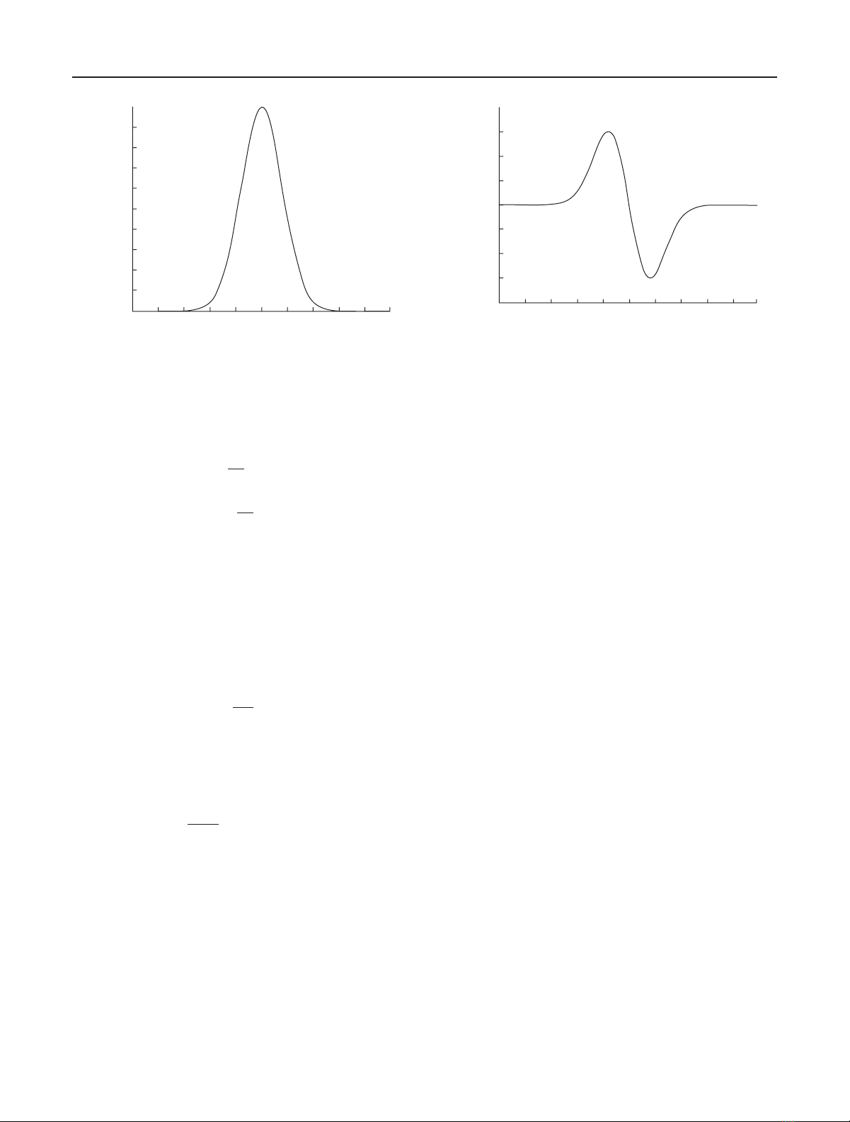
0.5
0.45
0.4
0.35
0.3
0.25
0.2
0.15
0.1
0.05
0
g(x,σ), σ=0.8
−5−4−3−2−10 1 2 3 4 5
x
Figure 1: The mask of the 1D OGHMs of order 0.
Property 1. Given a Gaussian function g(t,σ) and an image
f(x,y,t) of the image sequence {f(x,y,t)}t=0,1,2,...,wehave
Mnt,f(x,y,t)=
n
i=0
aidi
dtig(t,σ)∗f(x,y,t)
=n
i=0
aidi
dtig(t,σ)∗f(x,y,t),
(12)
where aidepends on σonly.
This property shows that the mask n
i=0ai(di/dti)g(t,σ)
of the nth moment is the linear combination of the Gaussian
function and its derivatives of different orders.
Property 2. Given a Gaussian function g(t,σ) and an image
sequence {f(x,y,t)}t=0,1,2,...,wehave
Mnt,f(x,y,t)=
k
i=0
a2id2i
dt2ig(t,σ)∗f(x,y,t)
for n=2k(nis even),
(13)
Mnt,f(x,y,t)
=
k
i=0
a2i+1d2i+1
dt2i+1 g(t,σ)∗f(x,y,t),
for n=2k+1(nis odd),
(14)
where aidepends on σonly.
This property shows that the mask of the OGHMs of odd
order is the linear combination of the derivatives of odd or-
ders of the Gaussian function, and the mask of the OGHMs
of even order is the linear combination of the derivatives of
even orders of the Gaussian function.
Property 3. Given a Gaussian function g(t,σ) and an image
sequence {f(x,y,t)}t=0,1,2,...,Mn(t,f(x,y,t)) =n
i=0ai(di/
0.8
0.6
0.4
0.2
0
−0.2
−0.4
−0.6
−0.8
(−2∗x/σ)∗g(x,σ), σ=0.8
−5−4−3−2−10 1 2 3 45
x
Figure 2: The mask of the 1D OGHMs of order 1.
dti)(g(t,σ)∗f(x,y,t)), we note that F(t,δ)=n
i=0ai(di/
dti)g(t,σ); then F(t,σ)=0hasndifferent real roots in the
interval (−∞,∞).
F(x,σ) is called the base function of the OGHMs (also
called the mask of the OGHMs). This property shows that
the mask of the nth moment has ndifferent zero crossings.
2.4. Some conclusions
From the properties of OGHMs, we see that these moments
are in fact linear combinations of the derivatives of the fil-
tered signal by a Gaussian filter. As it is well known, deriva-
tives are important features widely used in signal and im-
age processing. Because differential operations are sensitive
to random noise, a smoothing is in general necessary. The
Gaussian-Hermite moments just meet this demand because
of the Gaussian smoothing included. In image processing,
oneoftenneedsthederivativesofdifferent orders to effec-
tively characterize the images, but how to combine them is
still a difficult problem. The OGHMs show a way to construct
orthogonal features from different derivatives.
For facilely understanding the OGHMs, in Figures 1,2,3,
4,and5, we give out some characteristics charts of the base
function of OGHMs.
In the spatial domain, because the base function of the
nth-order OGHMs will change its sign ntimes, OGHMs can
well characterize different spatial modes as other orthogonal
moments. As to the frequency domain behavior, because the
base function of the nth-order OGHMs consists of more os-
cillations when the order nis increased, they will thus contain
more and more frequency. Tab l e 1 shows that the frequency
windows’ quality factor Q=(center/effective bandwidth) of
OGHMs base function is large than that of other moment
base function; therefore OGHMs separate different bands
more efficiently. Moreover, from the properties of OGHMs,
we see that these moments are in fact linear combinations
of the derivatives of the signal filtered by a Gaussian filter,
therefore, realizing differential operation and removing ran-
dom noise.
Orthogonal Moments and Their Applications 591
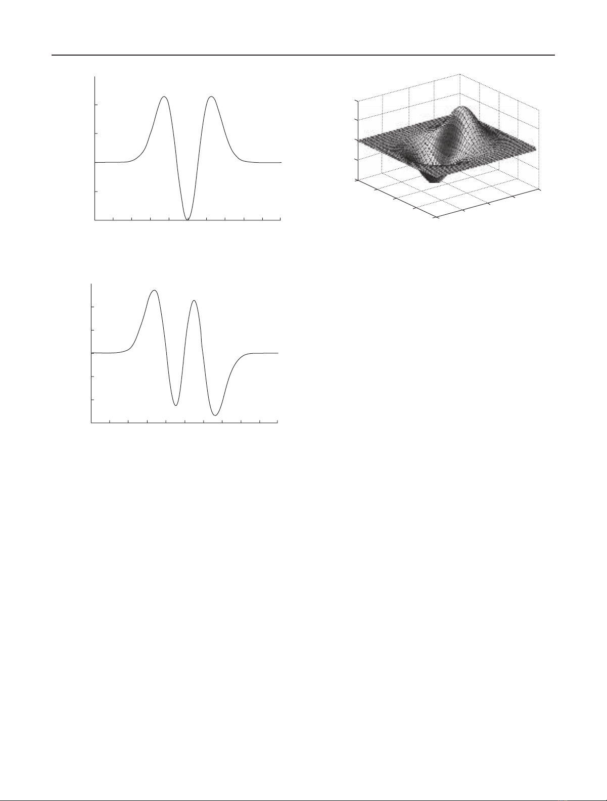
1.5
1
0.5
0
−0.5
−1
2nd (F(x,σ), σ=0.8)
−5−4−3−2−1012345
x
Figure 3: The mask of the 1D OGHMs of order 2.
3
2
1
0
−1
−2
−3
3rd (F(x,σ), σ=0.8)
−5−4−3−2−10 1 2 3 45
x
Figure 4: The mask of the 1D OGHMs of order 3.
From the viewpoint of frequency analysis, it seems that
the OGHMs characterize images more efficiently. With the
help of the technique representing frequency characteristics
by the band center ω0and effective bandwidth Be,wecanbet-
ter see the differences between the moment base functions.
In Tabl e 1, these characteristics for orders from 0 through 10
are shown. A similar conclusion holds in 2D cases. In general,
one uses the max order up to 10.
3. DETECTING MOVING OBJECTS USING OGHMS
3.1. Calculating the OGHMs images
According to (12), (13), and (14), we can see that all the
OGHMs are actually the linear combinations of the different
order derivatives of the image filtered by a temporal Gaus-
sian filter. As it is well known, the temporal derivatives can
be used to detect the moving objects in image sequences. The
OGHMs of odd orders are in fact the combinations of these
derivatives, it is therefore reasonable to use them to detect the
moving objects.
According to (12), Mnis equal to the temporal derivative
of the image filtered by a Gaussian filter, and the OGHMs
0.1
0.05
0
−0.05
−0.1
21
0
−1
−2−2−101
2
x
y
(−x/σ)g(x,y,σ), σ=0.8
Figure 5: The mask of the 2D OGHMs of order (1, 0).
are much smoother than other moments, therefore much less
sensitive to noise, which could facilitate the detection of the
moving objects in noisy image sequences.
To detect the moving objects by using the OGHMs, we
first calculate the temporal moments of an image sequence.
According to (14), calculating the temporal OGHMs of an
image sequence is equal to calculating the convolution of
the mask F(t,σ)with f(x,y,t). In order to approach the
mask F(t,σ), according to the inequality |t−Et|≥εg(t)dt ≤
(1/ε2)(t−Et)2g(t)dt =σ2/ε2,ifwetakeε=5σ, then
|t−Et|≥εg(t)dt ≤1/25 =4%. Hence the Gaussian function as
the convolution kernel is common to choose No=10σ+1,
namely the masks of size 2L+1withL=5σis used. For
practical computation reasons, we use only the moments of
orders up to 5. Hence, in order to detect the moving objects
using the OGHMs, the temporal OGHMs of an image se-
quence is calculated first.
Since both the positive values and negative values of the
moments correspond to the moving objects (containing the
noise), we take the absolute value of the moments instead of
their original values. For example, for Figure 6,fromFigure 7
to Figure 11, we present the OGHMs images, visualized by
linearly transforming the absolute value of the OGHMs to
the gray value ranging from 0 to 255. It can be seen that four
moving objects (2 persons, one car, and one cyclist) are well
enhanced in the moment images.
Thus M3contains more information than M1for de-
tecting the moving objects. Therefore, we can use the third
moment to detect the mobile objects. Figures 8and 9show
the experimental results in this case.
By comparing the results obtained in the case of σ=0.3
and σ=0.8,itcanbeseenwhenalargerσis used, the results
of the detection of the moving objects are less sensitive to the
noises, but the detected objects have larger sizes than their
real sizes. This phenomenon can be explained in Section 3.4.
The M5is a weighted sum of the first-, third-, and fifth-
order derivatives of image filtered by a temporal Gaussian fil-
ter. Therefore, M5still contains more information than these
M1and M3for the detection of the moving objects. Figures
10 and 11 show the experiment results.

592 EURASIP Journal on Applied Signal Processing
Table 1: Frequency characteristics of the base functions of geometric, Hermite, Legendre moments, and OGHMs.
Moment Geometric moment Hermite moment Legendre moment OGHMs
order ω0Beω0/Beω0Beω0/Beω0Beω0/Beω0Beω0/Be
00.40 2.11 0.1896 0.40 2.11 0.1896 0.40 2.11 0.1896 0.53 0.44 1.2045
11.25 3.87 0.3230 1.25 3.87 0.3230 1.25 3.87 0.3230 1.13 0.48 2.3542
21.59 4.71 0.3376 1.64 4.77 0.3438 1.94 4.90 0.3959 1.36 0.75 1.8133
32.32 5.74 0.4042 2.42 5.86 0.4130 2.60 5.74 0.4530 1.69 0.80 2.1125
42.61 6.23 0.4189 2.79 6.45 0.4326 3.25 6.46 0.5031 1.86 0.97 1.9175
53.28 7.00 0.4686 3.56 7.30 0.4877 3.92 7.15 0.5483 2.12 1.01 2.0990
63.52 7.36 0.4783 3.93 7.78 0.5051 4.59 7.77 0.5907 2.24 1.15 1.9478
74.15 7.98 0.5201 4.69 8.50 0.5518 5.29 8.41 0.6290 2.47 1.19 2.0756
84.36 8.27 0.5272 5.10 8.94 0.5705 6.01 9.01 0.6670 2.59 1.33 1.9474
94.95 8.79 0.5631 5.89 9.59 0.6142 6.77 9.64 0.7023 2.81 1.41 1.9929
10 5.14 9.03 0.5692 6.36 10.03 0.6341 7.55 10.23 0.7380 2.97 1.66 1.7892
3.2. Detecting the moving objects by integrating
the first, third, and fifth moments
It is known that the third and fifth moments contain more
information than the first moment, so we can integrate the
first, third, and fifth moments.
Because the first, third, and fifth moments are orthogo-
nal, one can consider that the first moment is the projection
of image f(x,y,t) on axis 1; the third moment is the pro-
jection of image f(x,y,t) on axis 3; the fifth moment is the
projection of image f(x,y,t) on axis 5; and the axes 1, 3,
and 5 are orthogonal. For getting the perfect real moving ob-
jects using the first, third, and fifth moments, we may use the
vector module of the 3D space to regain its actual measure,
namely M(x,y,t)=M2
1+M2
3+M2
5.
Henceforward, we principally adopt the M(x,y,t)as
OGHMs images (OGHMIs). We notice that the OGHMIs
contain more information than a single derivative image or
single OGHMs.
3.3. Segmenting the motion objects
We have noticed that OGHMI (OGHM) is also equal to the
image transformation. This transformation can suppress the
background, and enhance the motion information. We also
know, for the noise image, we cannot remove all noise by
a Gaussian filter. For obtaining the true region of the mov-
ing objects, having calculated the OGHMIs, we then detect
the moving objects by the use of the segmentation of such
images. To do this, a threshold for each OGHMI should
be determined. One of the well-known methods for the
threshold determination for image segmentation is the in-
variable moments method (IMM) [2,3,25]. But this method
has not taken into account the spatial and temporal rela-
tions between moving pixels, which are important for im-
age sequence analysis. To improve the method, instead of us-
ing a binary segmentation based on the threshold thus de-
termined, we use a fuzzy relaxation for the segmentation
of the moment images by taking into account these rela-
tions with the help of a nonsymmetric πfuzzy membership
function [2]:
πM(x,y); T,Mmin(x,y)
=
1−2T−M(x,y)2
T−Mmin(x,y)2
if 0 <T−M(x,y)
T−Mmin(x,y)≤0.5,
2T−M(x,y)
T−Mmin(x,y)−12
if 0.5<T−M(x,y)
T−Mmin(x,y)≤1,
1ifM(x,y)≥T,
0 otherwise,
(15)
where M(x,y) is the gray level of the OGHMI at the
point (x,y), Tis the segmentation threshold of the
moment image M(x,y), which is obtained by using
the (IMM) [2], Mmin(x,y) is the minimum of M(x,y).
π(M(x,y); T,Mmin(x,y)) is still noted as π(x,y).
For each point in the moment images, the membership
function, which gives a measure of the “mobility” of each
pixel in each moment image, is first determined. We then
apply a fuzzy relaxation to the membership function im-
ages, which gives the final results of the moving pixel detec-
tion [2].
3.4. Analyzing the localization errors
According to the theory of Gaussian filtering, a Gaussian
filter with larger standard deviation is less sensitive to the
noises, but brings larger localization errors [26]. How much
is the localization error of detecting the moving objects? Now
we give the discussion.
Let F(x,y,t)=(f(x,y,t)+n(x,y,t)) be the input image;
n(x,y,t) is the Gaussian white noise image; f(x,y,t) is the
true image at time t. Given the image F(x,y,t), the Gaussian


![Báo cáo seminar chuyên ngành Công nghệ hóa học và thực phẩm [Mới nhất]](https://cdn.tailieu.vn/images/document/thumbnail/2025/20250711/hienkelvinzoi@gmail.com/135x160/47051752458701.jpg)