Original
article
Estimation
of
total
yield
of
Douglas
fir
by
means
of
incomplete
growth
series
J
Bégin
JP
Schütz
1
Faculté
de
Foresterie
et
de
Géomatique,
Université
Laval,
Quebec
G1K
7P4;
Canada;
2
École
Polytechnique
Fédérale
de
Zurich,
ETH-Zentrum,
8092
Zurich,
Suisse
(Received
30
June
1993;
accepted
15
February
1994)
Summary -
This
study
establishes
and
validates
a
method
that
takes
into
account
yield
levels
and
permits
the
reconstruction
and
modelling
of
the
evolution
of
total
yield
based
on
incomplete
growth
series.
The
calculation
of
total
yield
of
Douglas
fir
(Pseudotsuga
menziesii
(Mirb)
Franco
var
menziesii
Franco)
is
carried
out
by
integrating
the
equation
of
volume
increment
per
metre
dominant
height
growth.
The
model
utilized
explains
94.8%
of
the
variation
in
volume
increment
per
metre
height
growth
of
the
14
experimental
plots.
The
evolution
of
total
yield
is
calculated
for
4
current
increment
levels.
The
concept
of
current
increment
levels
is
similar
to
the
concept
of
yield
levels,
and
corresponds
to
the
value
of
volume
increment
per
metre
height
growth,
at
a
height
of
30
m.
At
an
equivalent
yield
level,
the
calculated
total
yield
curves
correspond
closely
to
those
calculated
by
Bergel
(1985).
total
yield
/ yield
level
/ current
increment
level
/ volume
increment
/ Douglas
fir
Résumé —
Estimation
de
la
production
totale
du
Douglas
vert
au
moyen
de
séries
de
croissance
partielles.
Cette
étude
établit
et
valide
une
méthode
qui
tient
compte
de
niveaux
de
production
et
qui
permet
de
reconstituer
et
de
modéliser
l’évolution
de
la
production
totale
à
partir
de
séries
de
croissance
partielles.
Le
calcul
de
la
production
totale
du
Douglas
vert
(Pseudotsuga
menziesi
(Mirb)
Franco
var
menziesii
Franco)
s’effectue
en
intégrant
l’équation
de
l’accroissement
en
volume
par
mètre
d’accroissement
en
hauteur
dominante.
Le
modèle
utilisé
explique
94,8%
de
la
variation
de
l’accroissement
en
volume
par
mètre
d’accroissement
en
hauteur
des
14
placettes.
L’évolution
de
la
production
totale
est
calculée
pour
4
niveaux
d’accroissement
courant.
Le
concept
de
niveau
d’accroissement
courant
s’apparente
au
concept
de
niveau
de
production
et
correspond
à
la
valeur
de
l’accroissement
en
volume
par
mètre
d’accroissement
en
hauteur,
à
une
hauteur
de
30
m.
À
niveau
de
production
égal,
les
courbes
de
production
totale
calculées
correspondent
étroitement
à
celles
de
Bergel
(1985).
production
totale
/
niveau
de
production
/
niveau
d’accroissement
courant
/
accroissement
en
volume
/ Douglas
INTRODUCTION
For
decades,
yield
tables
have
served
as
a
basic
tool
for
forest
site
management.
In
the
European
context,
foresters
are
mainly
interested
in
total
yield,
ie
the
total
standing
volume
at
a
specific
moment
in
time,
to
which
one
adds
the
production
harvested
by
thinnings
since
the
stand
was
estab-
lished.
Classic
approach
The
classic
approach
to
modelling
total
yield
is
based
on
Eichhorn’s
extended
law,
which
states
that:
"the
total
crop
yield
is
without
exception
a
function
of
the
mean
height"
(Assmann,
1970).
Yield
levels
approach
Mitscherlich
(1953),
and
then
Assmann
(1954),
demonstrated
that
instead
of
a
single
relationship
between
total
yield
and
domi-
nant
height,
there
exist
several
relationships,
which
must
be
expressed
in
terms
of
differ-
ent
yield
levels.
Assmann
(1955)
termed
the
total
yield
attained
at
a
certain
dominant
height
as
the
general
yield
level
(allgemeine
Entragsniveau)
and
termed
the
variation
in
total
yield
within
the
same
site
index,
ie
for
a
specific
height-age
curve,
as
the
specific
yield
level
(spezielle
Ertragsniveau).
An
important
variability
in
total
volume
yield
was
also
reported
by
Schmidt
(1973)
for
Scots
pine
(Pinus
sylvestris
L),
Kennel
(1973)
for
beech
(Fagus
sylvaticus
L)
and
finally
Schütz
and
Badoux
(1979)
for
oaks
(Quercus petraea
Lieb and
Quercus
robur).
According
to
sereval
authors,
this
variability
can
be
as
high
as
14-25%
of
the
mean
value
(Assmann
and
Franz,
1965;
Kennel,
1973;
Schmidt,
1973;
Schütz
and
Badoux,
1979;
Bergel,
1985).
Estimation
by
means
of
incomplete
growth
series
In
the
absence
of
complete
growth
series,
Magin
(1963),
Prodan
(1965),
Decourt
(1967)
and
Decourt
and
Lemoine
(1969)
proposed
different
approaches
to
estimate
total
yield
from
plots
measured
only
once
or
from
growth
series.
These
are
generally
based
on
the
ratio
of
the
volume
of
the
mean
tree
harvested
by
thinning
to
that
of
the
mean
tree
remaining
on
the
site
(or
the
mean
tree
before
thinning).
However,
these
approaches
confound
the
yield
levels
and
thus
force
an
acceptance
of
the
validity
of
the
Eichhorn’s
law
(Eichhorn,
1904).
Faced
with
different
yield
levels,
the
cal-
culation
of
total
yield
imposes
methodolog-
ical
constraints
that
result
in
problems
for
researchers
who
have
only
incomplete
growth
series
(growth
series
for
which
the
volumes
from
the
first
thinnings
are
lack-
ing)
available
to
them.
This
situation
justi-
fies
the
development
of
an
alternative
approach
to
that
of
Assmann
and
Franz
(1963).
Objectives
The
objectives
of
this
study
are
to
establish
and
validate
a
method,
incorporating
yield
levels,
which
permits
the
reconstruction
and
modelling
of
the
evolution
of
total
yield
using
incomplete
growth
series.
The
study
con-
cerns
Douglas
fir
(Pseudotsuga
menziesii
(Mirb)
Franco
var
menziesii
Franco)
because
an
important
variability
in
yield
levels
has
been
observed
for
this
species
(Kramer,
1963;
Hamilton
and
Christie,
1971;
Bergel,
1985;
Christie,
1988).
MATERIALS
AND
METHODS
1
The
region
studied
extends
over
the
Swiss
plateau,
to
the
west
of
Zürich.
The
stands
of
Dou-
glas
fir
studied
are
found
on
the
flat
plain
or
on
hill-
sides,
at
altitudes
varying
between
450
and
750
m.
All
stands
are
included
in
vegetation
associa-
tions
of
beech
(Ellenberg
and
Klötzli,
1972).
Material
The
data
are
from
14
experimental
plots
of
the
Swiss
Federal
Institute
for
Forest,
Snow
and
Landscape
Research
of
Birmensdorf.
Of
these
plots,
8
were
established
at
the
beginning
of
the
century,
with
a
first
inventory
at
an
age
ranging
from
10
to
42
years.
The
6
other
plots
are
from
2
thinning
experiments
established
in
the
mid-six-
ties
and
measured
at
3
different
times.
Of
the
original
experimental
design,
we
retained
the
6
plots
where
the
thinning
intensity
best
corre-
sponded
to
that
of
the
older
stands
studied.
These
plots
were
measured
on
average
every
5
years.
At
each
sampling
time,
the
diameter
at
breast
height
of
all
stems
was
measured
with
a
precision
of
0.1
cm.
Observations
were
also
made
to
establish
the
height-diameter
relationship
serving
to
calculate
the
dominant
height
and
stem
volume
(top
diameter:
7
cm
over
bark)
of
trees.
A
comparison
with
data
from
Bergel’s
(1985)
table
indicates
that
these
14
experimental
plots
were
generally
subject
to
thinning
regimes
ranging
from
light
to
moderate.
The
site
index
values
(h
100
at
50
years)
vary
between
30.8
and
36.4
m
(x
=
33.2
m,
sx
=
1.4
m).
The
variation
in
the
estimate
of
site
index
of
each
plot,
as
a
function
of
age,
is
generally
not
more
than
±
1.5
m
once
the
period
of
juvenile
growth
has
terminated.
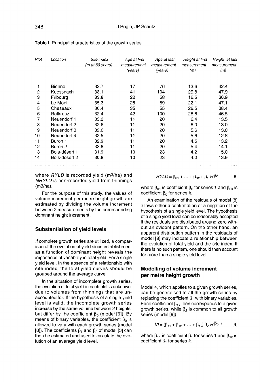
Table
I
pre-
sents
the
principal
characteristics
of
these
growth
series.
Methods
The
total
yield
corresponds
to
standing
volume
at
a
specified
time
to
which
is
added
the
sum
of
volumes
harvested
by
thinnings
since
stand
establishment.
It
is
also
expressed
as
the
sum
1
See
Bégin
(1992)
for
details
of
methods.
of
volume
increments
per
metre
height
growth.
Total
yield
is
then
calculated
by
integrating
the
equation
for
volume
increments
per
metre
height
growth
as
a
function
of
dominant
height
(equa-
tion
[1])
where
TYLD
is
total
yield
(m
3
/ha)
and
VI
is
volume
increment
per
metre
dominant
height
growth
(m
3
/ha/m).
Volume
increment
per
metre
dominant
height
growth
Volume
increment
per
metre
height
dominant
growth
(VI)
is
the
volume
increment
correspond-
ing
to
a
difference
of
1
m
of
dominant
height.
It
is
established
by
deriving
the
equation
for
total
yield
as
a
function
of
dominant
height
(equation
[2]).
Etter
(1949)
proposed
model
[3]
to
calculate
the
evolution
of
total
yield
from
a
complete
growth
series.
The
model
of
VI then
becomes
(model
[4]):
In
the
case
of
incomplete
growth
series,
the
total yield
curve
is
subject
to a downward
dis-
placement
equal
to
the
yield
not
accounted
for
in
thinnings
(NRYLD,
equation
[5]).
To
take
into
account
this
displacement,
a
constant
β
0
(model
6)
must
be
added
to
model
3
under
the
restriction
β
0
≤
0.
However,
this
constant
does
not
affect
the
derivative
of
the
equation
of
recorded
yield
(model
[7]),
which
provides
values
of
volume
increment
per
metre
height
growth
identical
to
those
obtained
by
model
[4].
In
fact,
the
non-recorded
yield
in
thinnings
does
not
affect
the
rate
of
change
in
vol-
ume
per
metre
at
a
given
height.
where
RYLD
is
recorded
yield
(m
3
/ha)
and
NRYLD
is
non-recorded
yield
from
thinnings
(m3/ha).
For
the
purpose
of
this
study,
the
values
of
volume
increment
per
metre
height
growth
are
estimated
by
dividing
the
volume
increment
between
2
measurements
by
the
corresponding
dominant
height
increment.
Substantiation
of
yield
levels
If
complete
growth
series
are
utilized,
a
compar-
ison
of
the
evolution
of
yield
since
establishment
as
a
function
of
dominant
height
reveals
the
importance
of
variability
in
total
yield.
For
a
single
yield
level,
in
the
absence
of
a
relationship
with
site
index,
the
total
yield
curves
should
be
grouped
around
the
average
curve.
In
the
situation
of
incomplete
growth
series,
the
evolution
of
total
yield
in
each
plot
is
unknown,
due
to
volumes
from
thinnings
that
are
un-
accounted
for.
If
the
hypothesis
of
a
single
yield
level
is
valid,
the
incomplete
growth
series
increase
by
the
same
volume
between
2
heights,
but
differ
by
the
coefficient
β
0
(model
[6]).
By
means
of
binary
variables,
the
coefficient
β
0
is
allowed
to
vary
with
each
growth
series
(model
[8]).
The
coefficients
β
1
and β
2
of
model
[3]
can
then
be
estimated
and
used
to
calculate
the
evo-
lution
of
an
average
yield
level.
where
β
01
is
coefficient
β
0
for
series
1
and
β
0k
is
coefficient
β
0
for
series
k.
An
examination
of
the
residuals
of
model
[8]
allows
either
a
confirmation
or
a
negation
of
the
hypothesis
of
a
single
yield
level.
The
hypothesis
of
a
single
yield
level
can
be
reasonably
accepted
if
the
residuals
are
distributed
around
zero
with-
out
an
evident
pattern.
On
the
other
hand,
an
apparent
distribution
pattern
in
the
residuals
of
model
[8]
may
indicate
a
relationship
between
the
evolution
of
total
yield
and
the
site
index.
If
there
is
no
such
pattern,
one
should
then
account
for
more
than
a
single
yield
level.
Modelling
of
volume
increment
per
metre
height
growth
Model
4,
which
applies
to
a
given
growth
series,
can
be
generalised
to
all
the
growth
series
by
replacing
the
coefficient β
1
with
binary
variables.
Each
coefficient
β
1k
then
corresponds
to
a
given
growth
series,
while
β
2
is
common
to
all
growth
series
(model
[9]).
where
β
11
is
coefficient
β
1
for
series
1 and
β
1k
is
coefficient
β
1
for
series
k.
The
approach
used
to
calculate
the
base-age
invariant
site
index
(Goelz
and
Burk,
1992)
appeared
adequate
to
model
the
evolution
of
curves
of
volume
increment
per
metre
height
growth.
This
approach
permits
the
modelling
of
volume
increment
per
metre
height
growth
inde-
pendently
of
the
reference
height.
Model
[10]
is
the
difference
form
of
the
model
9
based
on
solving
for
all
parameters
β
1
k.
VI
1
and
H1
repre-
sent
the
predictor
volume
increment
per
metre
height
growth
and
height,
respectively;
VI
2
rep-
resents
the
predicted
volume
increment
per
metre
height
growth
at
height
H2.
Levels
of
current
increment
The
evolution
of
curves
of
volume
increment
per
metre
height
growth,
taking
into
account
different
yield
levels,
resembles
in
some
ways
that
of
dom-
inant
height;
the
curves
have
a
common
origin
and
then
spread
out
progressively.
By
analogy
with
the
concept
of
general
yield
levels
of
Ass-
mann
(1955),
we
are
using
the
concept
of
levels
of
current
increment
to
characterize
each
curve
of
volume
increment
per
metre
height
growth.
More
specifically,
the
current
increment
level
is
the
value
of
volume
increment
per
metre
height
growth
corresponding
to
a
dominant
height
of
30
m.
This
reference
height
of
30
m
seems
to
be
appropriate
because
it
is
attainable
on
the
major-
ity
of
sites,
and
corresponds
approximately
to
the
mid-rotation
of
Douglas
fir.
Once
the
coefficient
β
2
is
calculated,
the
vol-
ume
increment
per
metre
height
growth
can
be
calculated
by
attributing
to
variables
VI
1
and
H1,
respectively,
the
values
of
currrent
increment
level
(CIL)
and
the
reference
height
of
30
m
(equation
[11 ]).
where
CIL
is
current
increment
level
(m
3
/ha/m).
Calculation
of
total
yield
curves
Integration
of
the
function
of
volume
increment
per
metre
height
growth
(equation
[11]),
for
a
given
current
increment
level,
gives
the
change
in
total
yield
between
2
heights.
Because
the
yield
in
Douglas
fir
stem
volume
(top
diameter:
7
cm
over
bark)
begins
only
at
a
dominant
height
of
4
m,
the
total
yield
can
be
calculated
at
a
given
dominant
height,
by
fixing
the
lower
limit
of
the
integral
at
4
m
(equation
[12]).
Validation
of
total
yield
curves
The
validation
of
the
equation
[12]
is
based
on
a
comparison
of results
with
the
total
yield
curves
of
Bergel
(1985).
The
latter
are
supported
by
a
large
data
base,
independent
of
the
data
utilized
in
the
present
study,
and
originate
from
a
geographic
region
that
is
comparable
to
that
of
the
present
study.
RESULTS
AND
DISCUSSION
Substantiation
of
yield
levels
The
evolution
of
recorded
yield
in
experi-
mental
plots
as
a
function
of
the
dominant
height
is
presented
in
figure
1.
The
plots
for
which
the
volumes
from
first
thinnings
are
lacking
are
represented
by
dashed
lines.
Differences
in
yield
levels
are
apparent
from
the
different
slopes
of
the
curves.
The
fit
of
observations
of
recorded
yield
from
model
[8]
appeared
at
first
view
to
be
excellent
(R
2
=
0.996,
se
=
62.1
m3
/ha;
table
II).
However,
the
plot-by-plot
examination
of
residuals
revealed
a
marked
pattern
in
prediction
errors,
as
well
as
significant
dis-
crepancies
as
great
as
250
m3
/ha
(fig
2).
The
observed
trends
indicate
that
the
vol-
ume
increment
per
metre
dominant
height
growth
of
plots
4
and
6
is
on
average
dif-
ferent
from
that of
plots
1
and
2
(fig
2).
This
distribution
of
residuals
demonstrates
that
a
model
incorporating
a
single
yield
level
can-
not
take
into
account
the
different
growth
rhythms
observed
in
the
experimental
plots.


%20--%3e%3cdefs%3e%3cstyle%3e%20.st0%20{%20fill:%20%23fff;%20}%20.st1%20{%20fill:%20%237800fa;%20}%20%3c/style%3e%3c/defs%3e%3cpath%20class='st1'%20d='M117.78,12.18H43.11c2.9,3.47,4.65,7.94,4.65,12.82,0,5.6-2.3,10.66-6.01,14.29h76.02l7.22-13.56-7.22-13.56Z'/%3e%3cg%3e%3cpath%20class='st0'%20d='M53.58,26.17h-.59v-1.46h.59v-4.96h2.83c1.78,0,2.67.94,2.67,2.82v5.76c0,1.87-.89,2.81-2.67,2.81h-2.83v-4.96ZM55.36,21.37v3.34h1.1v1.46h-1.1v3.34h1.01c.61,0,.91-.37.91-1.1v-5.93c0-.74-.3-1.1-.91-1.1h-1.01Z'/%3e%3cpath%20class='st0'%20d='M65.99,31.14h-1.8l-.31-2.07h-2.19l-.31,2.07h-1.64l1.82-11.39h2.62l1.82,11.39ZM65.28,18.04c-.25.46-.51.77-.75.94-.21.15-.47.22-.79.22-.26,0-.57-.07-.92-.22l-.38-.15c-.14-.05-.26-.07-.37-.07-.3,0-.53.18-.71.54l-.91-.68c.25-.46.51-.77.75-.94.21-.14.48-.21.79-.21.26,0,.57.07.92.21l.38.15c.14.05.26.07.37.07.3,0,.53-.18.71-.54l.91.68ZM61.91,27.52h1.73l-.87-5.76-.87,5.76Z'/%3e%3cpath%20class='st0'%20d='M74.53,26.89v1.52c0,1.91-.89,2.86-2.67,2.86s-2.67-.95-2.67-2.86v-5.93c0-1.91.89-2.86,2.67-2.86s2.67.95,2.67,2.86v1.11h-1.69v-1.22c0-.75-.31-1.12-.93-1.12s-.93.37-.93,1.12v6.15c0,.74.31,1.11.93,1.11s.93-.37.93-1.11v-1.63h1.69Z'/%3e%3cpath%20class='st0'%20d='M81.4,31.14h-1.8l-.31-2.07h-2.19l-.31,2.07h-1.64l1.82-11.39h2.62l1.82,11.39ZM75.9,19.2l1.52-1.91h1.71l1.51,1.91h-1.61l-.76-.95-.75.95h-1.61ZM77.32,27.52h1.73l-.87-5.76-.87,5.76ZM83.1,15.99l-1.76,1.91h-1.26l1.17-1.91h1.86Z'/%3e%3cpath%20class='st0'%20d='M84.86,19.75c1.78,0,2.67.94,2.67,2.82v1.48c0,1.87-.89,2.81-2.67,2.81h-.85v4.28h-1.79v-11.39h2.64ZM84.01,21.37v3.86h.85c.58,0,.87-.36.87-1.08v-1.71c0-.71-.29-1.07-.87-1.07h-.85Z'/%3e%3cpath%20class='st0'%20d='M93.51,19.75c1.78,0,2.67.94,2.67,2.82v1.48c0,1.87-.89,2.81-2.67,2.81h-.85v4.28h-1.79v-11.39h2.64ZM92.66,21.37v3.86h.85c.58,0,.87-.36.87-1.08v-1.71c0-.71-.29-1.07-.87-1.07h-.85Z'/%3e%3cpath%20class='st0'%20d='M98.8,31.14h-1.79v-11.39h1.79v4.88h2.03v-4.88h1.83v11.39h-1.83v-4.88h-2.03v4.88Z'/%3e%3cpath%20class='st0'%20d='M105.36,24.55h2.46v1.62h-2.46v3.34h3.09v1.63h-4.88v-11.39h4.88v1.63h-3.09v3.18ZM108.17,17.29l-1.76,1.91h-1.26l1.17-1.91h1.86Z'/%3e%3cpath%20class='st0'%20d='M112.2,19.75c1.78,0,2.67.94,2.67,2.82v1.48c0,1.87-.89,2.81-2.67,2.81h-.85v4.28h-1.79v-11.39h2.64ZM111.35,21.37v3.86h.85c.58,0,.87-.36.87-1.08v-1.71c0-.71-.29-1.07-.87-1.07h-.85Z'/%3e%3c/g%3e%3ccircle%20class='st1'%20cx='25'%20cy='25'%20r='20'/%3e%3cpath%20class='st0'%20d='M32.78,19.27c2.92,0,4.43,2.55,5.28,5.33l.71,2.17c.14.38-.33.75-.71.75h-5.61c.19-.33.24-.71.09-1.08l-.75-2.45c-.43-1.32-.99-2.64-1.79-3.77.75-.57,1.65-.94,2.78-.94h0ZM25,18.38c3.25,0,4.9,2.78,5.89,5.89l.76,2.45c.14.42-.33.8-.8.8h-11.69c-.42,0-.94-.38-.8-.8l.75-2.45c.99-3.11,2.64-5.89,5.89-5.89h0ZM25,11.35c1.74,0,3.11,1.37,3.11,3.11s-1.37,3.11-3.11,3.11-3.11-1.41-3.11-3.11,1.41-3.11,3.11-3.11h0ZM17.27,19.27c1.08,0,1.98.38,2.73.94-.8,1.13-1.37,2.45-1.74,3.77l-.8,2.45c-.14.38-.05.75.09,1.08h-5.56c-.42,0-.9-.38-.75-.75l.71-2.17c.9-2.78,2.41-5.33,5.33-5.33h0ZM17.27,12.91c1.51,0,2.78,1.27,2.78,2.83s-1.27,2.83-2.78,2.83-2.83-1.27-2.83-2.83,1.27-2.83,2.83-2.83h0ZM32.78,12.91c1.56,0,2.78,1.27,2.78,2.83s-1.23,2.83-2.78,2.83-2.83-1.27-2.83-2.83,1.27-2.83,2.83-2.83h0ZM27.07,28.56v.09c0,.57-.24,1.08-.61,1.46h0v.05c-.38.33-.9.57-1.46.57s-1.08-.24-1.46-.61h0c-.38-.38-.61-.9-.61-1.46v-.09h1.41v.09c0,.19.05.38.19.47v.05c.09.09.28.19.47.19s.38-.09.47-.19v-.05c.14-.09.24-.28.24-.47t-.05-.09h1.41ZM30.99,28.56v.09c0,1.65-.66,3.16-1.74,4.24-1.08,1.08-2.59,1.79-4.24,1.79s-3.16-.71-4.24-1.79l-.05-.05c-1.04-1.08-1.7-2.55-1.7-4.2v-.09h1.41v.09c0,1.27.47,2.4,1.27,3.25h.05c.85.85,1.98,1.37,3.25,1.37s2.4-.52,3.25-1.37c.85-.8,1.37-1.98,1.37-3.25v-.09h1.37ZM34.99,28.56v.09c0,2.78-1.13,5.28-2.92,7.07-1.79,1.79-4.29,2.92-7.07,2.92s-5.23-1.13-7.07-2.92c-1.79-1.79-2.92-4.29-2.92-7.07v-.09h1.41v.09c0,2.4.94,4.53,2.5,6.08,1.56,1.56,3.72,2.5,6.08,2.5s4.52-.94,6.08-2.5c1.56-1.56,2.5-3.68,2.5-6.08v-.09h1.41Z'/%3e%3c/svg%3e)