ISSN 1859-1531 - TẠP CHÍ KHOA HỌC VÀ CÔNG NGHỆ - ĐẠI HỌC ĐÀ NẴNG, VOL. 22, NO. 9A, 2024 77
ENHANCED FORCE FIELD CONSTRUCTION FOR GRAPHENE MONOLAYERS
VIA NEURAL NETWORK-BASED FITTING OF DENSITY FUNCTIONAL
THEORY DATA
XÂY DỰNG TRƯỜNG LỰC NÂNG CAO CHO CÁC LỚP ĐƠN GRAPHENE BẰNG CÁCH
ĐIỀU CHỈNH DỮ LIỆU LÝ THUYẾT HÀM MẬT ĐỘ DỰA TRÊN MẠNG NƠ-RON
Tan-Tien Pham1, Tien B. Tran2, Viet Q. Bui1*
1The University of Danang - Advanced Institute of Science and Technology, Vietnam
2The University of Danang, Vietnam
*Corresponding author: bqviet@ac.udn.vn
(Received: May 23, 2024; Revised: July 22, 2024; Accepted: September 24, 2024)
Abstract - This study presents a novel neural network (NN)
framework for developing force fields specific to graphene
monolayers, utilizing data obtained from first-principles
calculations. The authors analyze three primary force
components, force magnitude and the cosines of two angles
across different configurations of surrounding carbon atoms.
Initially, the NN applied to the three nearest neighbors, achieving
average absolute testing errors of 0.375 eV/Å, 0.092, and 0.085
for the respective components. Then, expanding the input
variables to nine surrounding atoms, which significantly
enhances the precision of the force field models, reducing the
error in force magnitude to approximately 1%. This improvement
represents a 33% to 59% increase in accuracy over the initial
method. The results demonstrate the potential of NNs to generate
highly accurate force fields for graphene.
Tóm tắt - Nghiên cứu này giới thiệu một mô hình mạng nơ-ron
(NN) mới để phát triển trường lực được thiết kế cho các lớp đơn
graphene, sử dụng dữ liệu được tính toán từ nguyên lý thứ nhất.
Ba thành phần lực chính được phân tích gồm: độ lớn của lực và
cosin của hai góc được đo trên các cấu hình khác nhau của các
nguyên tử carbon xung quanh. Ban đầu, áp dụng NN cho ba
nguyên tử lân cận gần nhất, với các sai số kiểm tra tuyệt đối trung
bình lần lượt là 0,375 eV/Å, 0,092 và 0,085 cho các thành phần
tương ứng. Sau đó, mở rộng các biến đầu vào bao gồm chín
nguyên tử xung quanh, điều này đã cải thiện đáng kể độ chính xác
của mô hình trường lực, giảm sai số độ lớn lực xuống còn khoảng
1%. Sự cải thiện này tương đương với mức tăng độ chính xác từ
33% đến 59% so với phương pháp ban đầu. Kết quả cho thấy,
tiềm năng của NN trong việc tạo ra các trường lực có độ chính
xác cao cho graphene.
Keywords - Graphene; force field; neural network
|𝐹
|
.
Từ khóa - Graphene; force field; neural network
|𝐹
|
.
1. Introduction
In the past decade, significant interest has been devoted
to study two-dimensional materials, especially graphene [1].
Such material continues to highly attract attention due to its
unique thermodynamic and electronic properties. In this
honeycomb structure, carbon atoms are linked together by
sp2-hybridized bonds, which provide remarkable
mechanical stability and unusually high thermal
conductivity at the nanoscale [2, 3]. Therefore, investigating
the thermal properties of graphene is considered an
important and challenging task, which has been addressed
using various experimental and theoretical approaches. In
this study, our objective is to develop a force-field (FF)
acting on a C atom infinite graphene monolayer by adopting
an efficient numerical fitting strategy.
Density Functional Theory (DFT) has been extensively
utilized to calculate electronic structure and properties of
materials due to its balance between accuracy and
computational efficiency. DFT allows for the
determination of total energies, electronic densities, and
forces acting on atoms, which are crucial for developing
reliable force fields. By employing DFT calculations, the
authors can accurately capture the interactions within the
graphene monolayer, providing a solid foundation for
constructing precise neural network-based force fields.
In reality, graphene is hardly found in its equilibrium
ground state, and the force acting on each C atom is
different from case to case, which highly depends on the
environment of interactions with other surrounding C
atoms. In order to clearly understand the heat spreading
process in graphene, molecular dynamics simulations
should be executed with a reliable FF. However, using ab
initio FF in direct Born-Oppenheimer dynamics is too
computationally demanding and thus unrealistic.
Significant efforts have been made to construct FFs for
graphene using empirical approaches, such as using
Tersoff's valence force model to describe sp2 interactions
[4], followed by Monte Carlo simulations to estimate
important thermodynamic quantities such as Young's
modulus and molar heat capacity [5]. Recently, efforts
have been made to construct an in-plane FF for graphene
based on first-principles calculation data [6]. In this study,
the authors present a new approach to interpolate FFs for
graphene by employing the neural network (NN) technique
[7] for direct force fitting.
As a powerful and robust tool for function fitting with
high accuracy, for years, artificial NN has been widely
applied to develop Potential Energy Surfaces (PES) by
fitting electronic structure data [8, 9, 10]. The most obvious
disadvantage of the NN method is the requirement of large
dataset for fitting processes. Recently, there have been
contributions to reduce the amount of required data by
developing a function-gradient simultaneous fitting
procedure, which is termed combined-function-derivative

78 Tan-Tien Pham, Tien B. Tran, Viet Q. Bui
approximation [11]. Also, the NN architecture was
modified to allow the direct permutation of atoms of
similar identity in a molecular system [12]. Depending
upon the complexity of molecular systems, the algorithm
for NN symmetry adaptation may vary.
The graphene monolayer investigated herein is quite
complex, and the development of a global many-body
PES would be very computational demanding and may be
an unrealistic task. In fact, not the total energy, but
the force acting on each C in the graphene network is
realized as the major concerning quantities in molecular
dynamics simulations. Therefore, a reliable FF of
graphene is crucial and should be considered as a priority
task in investigating the thermal property of graphene. In
this study, the authors employ feed-forward NNs to
develop a direct FF for graphene monolayer. Three
strategies of fitting with ascending NN size are presented
in order to evaluate the influence of C atoms on the FF.
Such approach is necessary to understand the role of force
acting on each C atom in a graphene monolayer.
The present result is useful for quickly and accurately
building the PES, which play an important role in
graphene studies.
2. FF developing procedure
2.1. Description of geometry representation
In a large-scale graphene monolayer with thousands
of C atoms, it is more beneficial to approximate the force
acting on each individual C atom directly rather than to
develop a full PES for the whole graphene sheet, which
only allows indirect extractions of forces. The force
acting on each C atom can be approximated by
performing NN fitting, in which the internal variables
defining relative positions of the surrounding atoms are
used as input variables and the force components are used
as targeted output.
As illustrated in Figure 1, the currently-considered C
atom has direct interactions via sp2 bonds with three
surrounding atoms, which are denoted as C1, C2, and C3.
For convenience of NN fitting, C1 is chosen in such a way
that it establishes the shortest C-C bond with C0 among
three nearest neighbor atoms, while C3 gives the longest
C-C bond distance with C0. To describe the relative
positions of C1, C2, and C3 with respect to C0, the authors
employ the internal coordinate system (bond distances,
bending and dihedral angles) as given in Table 1.
The completeness of long-range interaction may be
enhanced by further expanding the surrounding
environment and extending the set of FF input
parameters. By doing this, the authors consider the long-
range interaction effects on the center C atom, and
supposingly add more correction terms to FF function.
Specifically, this is done by further considering the
relative positions of six additional C atoms, which are
denoted as C4,..., C9 in Figure 1. In our model, C4 and C5
have direct interactions with C1, C6 and C7 have direct
interactions with C2, while C4 and C5 bond directly to C3.
The internal-coordinate descriptions of those following C
atoms are given in Table 1.
Table 1. Internal variables (bond distances (Å) and angles (o))
that define the relative positions of nine surrounding C atoms
Input variable
Description
Minimum
Maximum
r1
C0-C1
1.219
1.526
r2
C0-C2
1.271
1.594
r3
C0-C3
1.349
1.737
r4
C1-C4
1.219
1.588
r5
C1-C5
1.289
1.737
r6
C2-C6
1.219
1.594
r7
C2-C7
1.271
1.737
r8
C3-C8
1.219
1.576
r9
C3-C9
1.297
1.737
Θ1
C2-C0-C1
101.799
139.372
Θ2
C3-C0-C1
101.818
137.031
Θ3
C4-C1-C0
101.799
139.168
Θ4
C5-C1-C0
100.778
141.919
Θ5
C6-C2-C0
101.799
139.372
Θ6
C7-C2-C0
101.682
142.127
Θ7
C8-C3-C0
100.778
142.127
Θ8
C9-C3-C0
101.818
140.479
Φ1
C3-C0-C1-C2
123.828
180.000
Φ2
C4-C1-C0-C2
0.000
180.000
Φ3
C5-C1-C0-C2
0.000
180.000
Φ4
C6-C2-C0-C1
0.000
180.000
Φ5
C7-C2-C0-C1
0.000
180.000
Φ6
C8-C3-C0-C1
0.000
180.000
Φ7
C9-C3-C0-C1
0.000
180.000
Figure 1. The geometry configuration for FF construction: one
center and nine surrounding C atoms. The force vector |𝐹
| is
decomposed into three major components: force magnitude
(|𝐹
|), Θ and Φ. For the uniqueness of a configuration, the order
of (C
1
, C2, C3) is chosen in such a way that C0C1 is the shortest,
while C0C3 is the longest bond
In the conventional PES development with NN fitting,
the output is a single quantity, which solely represents the
total energy. In this study, the NN method is employed to
predict the force vector |𝐹
| acting on a particular C atom
instead of energy. The force vector, however, cannot be
represented by a single quantity; in fact, it must be
fragmented into three components which precisely reveal
the magnitude and orientation of |𝐹
|: force magnitude
(|𝐹
|), cosine of the bending angle between vectors |𝐹
| and
C0C1 (cos(Θ)), and cosine of the dihedral angle defined by
vectors |𝐹
|, C0C1, and C1C2 (denoted as cos(Φ)). A precise

ISSN 1859-1531 - TẠP CHÍ KHOA HỌC VÀ CÔNG NGHỆ - ĐẠI HỌC ĐÀ NẴNG, VOL. 22, NO. 9A, 2024 79
pictorial illustration of |𝐹
|, cos(Θ) and cos(Φ) is presented
in Figure 1.
In our developing procedure, it is necessary to build a
database which describes the orientations of atoms (inputs)
and forces (targeted outputs) based on electronic structure
calculations. Subsequently, the numerical NN fitting
method is employed to fit the database and produce an
approximate force field.
2.2. Electronic structure calculations
The electronic structure calculations in this study for
force-field sampling are executed by first-principles
calculations based on density functional theory (DFT) [13,
14], as implemented in the Quantum Espresso package
[15]. In particular, the Perdew-Burke-Ernzerhof (PBE)
exchange-correlation functional [16, 17] within the
generalized gradient approximation is employed to
calculate total energies of the graphene supercell with the
Vanderbilt ultrasoft pseudopotential for C atoms [18, 19].
Structural data are obtained by performing sample Born-
Oppenheimer molecular dynamics with one restriction that
the Brillouin zone is only represented by the point. The
kinetic-energy cut-off of 45 Rydberg (612 eV) is chosen
for plane-wave expansions.
To sample data points for fitting purposes, the authors
perform Born-Oppenheimer molecular dynamics at 1500
K for a graphene supercell consisting of 32 C atoms. Due
to periodicity of the graphene sheet, in each step during the
MD trajectory, the authors are able to extract 32
configurations by considering each C atom as the center
atom. In total, after nearly 5,000 MD steps, the database is
constructed with 157,792 configurations.
Figure 2. Data distributions of three force components (|𝐹
|,
cos(Θ) and cos(Φ)). N represents the number of configurations
in a particular range
For reducing computational feasibility and attaining
higher efficiency in NN training, it is necessary to reduce
the database by making a random selection of 55,726
configurations from the initial database. Hence, in most of
the NN fits discussed below, the training set is constituted
by 55,726 configurations, while an independent set of
2,786 configurations is randomly chosen to construct the
testing set for validation purposes. The ranges of three
output components in the training set consisting of 55,726
data points are given in Table 2. In Figure 2, the statistical
distributions of three force components are shown. It can
be seen clearly that forces with low magnitude (near
equilibrium region, from 0 to 3 eV/Å) dominates. Since
C0C1 is chosen as the shortest C-C bond around C0, |𝐹
| has
a higher tendency to be opposite to the C0C1 vector. As a
result, more values around the -180o region are obtained for
Θ. Overall, the authors believe that a sufficient number of
configurations has been sampled to explicitly describe
three output components.
Table 2. Minimum and maximum values of three output
components
Output components
Minimum
Maximum
|𝐹
|
(e
V/Å)
0.081
14.508
cos(Θ)
-1.000
1.000
cos(Φ)
-1.000
1.000
2.3. Neural network fitting method
Two-layer feed-forward NNs, which can be consulted
from Hagan et al. [7], are employed to approximate the FF
data in this study. As mentioned earlier, such an NN
architecture is widely utilized in constructing PES for gas-
phase molecular as well as condensed-matter systems.
Initially, the input and target data are scaled from -1 to 1 to
enhance the training effectiveness. For convenience, the
authors generally denote input as p and targeted output as
t. The scaling technique is done as following.
𝑝 = 2(𝑝𝑖−𝑝𝑖
𝑚𝑖𝑛)
𝑝𝑖
𝑚𝑎𝑥−𝑝𝑖
𝑚𝑖𝑛 − 1 for i = 1,…,24 (1)
𝑡𝑖
𝑠𝑐𝑎𝑙𝑒𝑑 = 2(𝑡𝑖−𝑡𝑖
𝑚𝑖𝑛)
𝑡𝑖
𝑚𝑎𝑥−𝑡𝑖
𝑚𝑖𝑛 − 1 for i = 1, 2, 3 (2)
where 𝑝𝑖
𝑚𝑖𝑛 and 𝑝𝑖
𝑚𝑎𝑥 respectively represent the minimum
and maximum values of the 𝑖𝑡ℎ input parameter, while 𝑡𝑖
𝑚𝑖𝑛
and 𝑡𝑖
𝑚𝑎𝑥 denote the minimum and maximum values of the
𝑖𝑡ℎ output parameter. Mathematically, this scaling
technique is meaningful because it helps to reduce input
and output data ranges for numerical fitting; moreover, it
should be noticed that such a technique also makes
physical units vanish. As can be seen from Table 1, the
ranges of the second and third output parameters (cos(Θ))
and third (cos(Φ)), respectively are almost [-1; 1].
Therefore, the above scaling technique does not have
significant impacts on those values; however, for
consistency of the overall procedure, scaling is still applied
to those two output quantities.
Subsequently to scaling, the n scaled inputs are
introduced into the first (input) layer and processed by the
hidden layer, then finally m outputs in the last layer are
produced. An illustration for the operating principle of a
typical feed-forward NN is introduced in Figure 3. n scaled
inputs are processed by M hidden neurons in the first layer
to produce M intermediate values using the following
equation:
𝑥𝑖= 𝑓(∑𝑤1𝑖,𝑗𝑝𝑗
𝑠𝑐𝑎𝑙𝑒𝑑 + 𝑏1𝑗
𝑛
𝑗=1 ) for i = 1,…,M
where 𝑤1 is an M×n matrix identified as the first weight
matrix, 𝑏1 is an M×1 column vector representing the bias
values of the first layer, and f is the transfer function. In
this study, the authors employ the hyperbolic tangent
function as the transfer function in the first layer. Hornik et

80 Tan-Tien Pham, Tien B. Tran, Viet Q. Bui
al. [20] showed that the utilization of a sigmoid function in
the hidden layer could make a NN an universal
approximator for analytic functions.
The final output quantities T are subsequently
calculated by employing a linear function to combine all x
values as:
𝑇𝑙=∑𝑤2𝑘,𝑙𝑥𝑘+ 𝑏2𝑙
𝑀
𝑘=1 for l = 1,…,m
In the above equation, 𝑤2 is an m×M matrix, 𝑏2 is an m×1
vector, which represent the weight and bias values of the
second layer, respectively. In our case, T consists of three
quantities, which represent the scaled force components
(targeted outputs).
Figure 3. The feed-forward NN model for FF fitting
3. Results and discussions
Traditionally, the NN output for PES fitting consists of
one single value; however, the description for a force
vector requires that at least three parameters get involved
as stated in Figure 1. As a result, the fitting process in this
study is more complicated. In fact, the authors suggest
three strategies to obtain well-fitted FFs using the NN
method. In the first strategy, (1) the authors only consider
three surrounding C atoms to have impacts on the force
acting on C0; in other words, six input variables (r1, r2, r3,
1, 2 and 1), which fully describe the relative positions of
(C1, C0, C3), will be taken into account. Hence, a feed-
forward NN with six input signals will be employed to
predict three components of the force. In the second
approach, (2) the authors consider nine surrounding C
atoms to have impacts on the magnitude of the force acting
on C0 (|𝐹
|) and cos(Θ), while the prediction of cos(Φ) is
attributed by considering three nearest neighbors.
Therefore, two different NNs need to be constructed: one
NN reading all 24 input signals will be employed to fit |𝐹
|
and cos(Θ), while another NN reading 6 input signals will
be employed to predict the last output quantity, cos(Φ). In
the last approach, (3) a highly-complex NN operating on
24 input signals will be employed to fit the three outputs
simultaneously.
3.1. NN FF with six input signals
As mentioned earlier, three components of a force
vector (|𝐹
|) are predicted by considering the influence of
only three surrounding carbon atoms. Potentially, there is
an advantage when this strategy is used, i.e. the number of
involving variables in the FF function will be highly
reduced. Compared to the full utilization of nine
surrounding C atoms (which results in a total number of
24 input variables), in this case, only six input variables are
introduced into the first layer of a feed forward NN.
Because of lower numbers of input variables, the size of
NN parameters (weight and bias values) in this case would
be significantly smaller. As a result, the training process
consumes less computational time. In addition, it is also
more advantageous to extract the force from the NN
function.
The FF is fitted with NNs that have various numbers of
hidden neurons (from 10 to 35 neurons). At this point, the
root-mean-squared error (rmse) and average-absolute error
(aae) are determined for the training and testing sets for
statistical accuracy evaluation. As shown in Table 2, with
only 10 neurons in the hidden layer, the testing rmse and
aae for |𝐹
| of the training set are 0.480 and 0.381 eV/Å,
respectively. Compared to the maximum of |𝐹
| in the
database (14.51 eV/Å), the ratio of 𝑎𝑎𝑒/|𝐹
| is about
2.63%. For convenience, the rmse and aae of three outputs
given by six different NN FFs are summarized in Table 3.
It can be observed that the training rmse and aae for cos(Θ)
and cos(Φ) are relatively large compared to their maximum
values (1.00) when the NN is constructed with 10 neurons.
Table 3. Training (and testing) rmse and aae of
the fitted NN FFs which process six input signals
Number of
neurons
10
15
20
25
30
35
rmse
|𝐹
|
(eV/Å)
0.480
0.476
0.475
0.474
0.473
0.472
(0.480)
(0.471)
(0.473)
(0.472)
(0.477)
(0.470)
cos (Θ)
0.161
0.156
0.155
0.153
0.153
0.153
(0.161)
(0.152)
(0.152)
(0.151)
(0.153)
(0.147)
cos (Φ)
0.179
0.178
0.176
0.176
0.175
0.175
(0.177)
(0.161)
(0.171)
(0.169)
(0.184)
(0.167)
aae
|𝐹
|
(eV/Å)
0.381
0.378
0.377
0.376
0.376
0.376
(0.381)
(0.375)
(0.378)
(0.375)
(0.380)
(0.375)
cos (Θ)
0.104
0.100
0.099
0.097
0.097
0.096
(0.106)
(0.100)
(0.098)
(0.096)
(0.099)
(0.092)
cos (Φ)
0.093
0.092
0.091
0.090
0.090
0.089
(0.093)
(0.088)
(0.088)
(0.089)
(0.093)
(0.085)
Figure 4. Training errors (rmse and aae) vs. number of
hidden neurons from NN fitting with six input variables
In Figure 4, the authors show the fitting performance of
|𝐹
|, which is revealed by the rmse and aae of training and
testing data, with respect to the number of hidden neurons.

ISSN 1859-1531 - TẠP CHÍ KHOA HỌC VÀ CÔNG NGHỆ - ĐẠI HỌC ĐÀ NẴNG, VOL. 22, NO. 9A, 2024 81
As the number of hidden neurons increases from 10 to 35,
it is statistically observed that the fitting quality of both
training and testing sets is not significantly improved. For
cos(Θ) and cos(Φ) fitting, it is also the case as the
utilization of 35 hidden neurons does not result in
significant change in the overall accuracy. Therefore, the
authors believe that the FF is not well interpolated if only
six input variables are considered in NN constructions. In
other words, the physical picture of C-C interactions is not
well described when the authors only consider the
influence of three surrounding C atoms. Hence, NN fitting
attains its fitting limit regardless of hidden neuron
numbers.
3.2. The combination of two feed-forward NNs to fit the FF
In this approach, the authors combine two feed-forward
NNs to represent the FF. All 24 input parameters
describing relative positions of nine surrounding C atoms
are used as the input layer for the first NN, which is
employed to handle two force components (|𝐹
| and
cos(Θ)). The number of hidden neurons for this NN ranges
from 50 to 125. In the second NN to fit the last force
component (cos(Φ)), the input layer only consists of six
variables. For convenience, the statistical fitting errors of
the first and second NNs are shown in Table 4.
Table 4. Training (and testing) rmse and aae of the combination
of two feed-forward NNs
Number of neurons
50
75
100
125
rmse
|𝐹
|
(e
V/Å)
0.206
(0.208)
0.200
(0.202)
0.195
(0.196)
0.193
(0.192)
cos(Θ)
0.087
(0.086)
0.085
(0.085)
0.082
(0.083)
0.082
(0.080)
cos(Φ)
0.173
(0.174)
0.173
(0.163)
0.173
(0.182)
0.173
(0.171)
aae
|𝐹
|
(e
V/Å)
0.162
(0.163)
0.156
(0.160)
0.153
(0.154)
0.151
(0.151)
cos(Θ)
0.055
(0.055)
0.054
(0.053)
0.053
(0.052)
0.052
(0.052)
Number of neurons
25
30
45
50
rmse
cos(Φ)
0.173
(0.174)
0.173
(0.163)
0.173
(0.182)
0.173
(0.171)
aae
0.087
(0.086)
0.087
(0.086)
0.087
(0.090)
0.088
(0.086)
Recall that in the first approach, when the number of
hidden neurons increases from 50 to 125, training and
testing rmse and aae drop slowly. Compared to the rmse
and aae in the previous stage, it can be seen that the fitting
quality of |𝐹
| and cos(Θ) is improved. As shown in Table
4, when the FF is fitted with 125 hidden neurons, the
authors obtain the best rmse and aae for both training and
testing sets. The third force component fitting is executed
using NNs with 25-50 hidden neuron, and no significant
improvements can be observed in the second NN for
cos(Φ) prediction. Compared to the results using the first
fitting strategy presented above, the current aae produced
by a 30-hidden-neuron NN is improved by 3%. When the
NN size increases to 45-50 neurons, the aae does not drop
as expected.
By performing such fitting trials, the authors are able to
interpret the physical characteristics of the dihedral angle
in the system. Even when cos(Φ) is treated separately with
a feed-forward NN, the fitting accuracy does not
significantly increase. Thus, the six chosen input variables
are still not sufficient to describe the true behavior of the
third force component. This means that it highly depends
on the interaction environment, as will be proved in the
third approach to fit the FF shown below.
3.3. NN FF with 24 input signals
In the last approaching strategy, all 24 input parameters
which describe the relative positions of nine surrounding C
with respect to the center C atom jointly constitute the input
layer of the NN FF. At this stage, the number of hidden
neurons ranges from 50 to 125. As the authors evaluate the
training and testing errors (both rmse and aae), this approach
possesses the most promising fitting ability because of its
best accuracy compared to the previous NN fits. With 50
hidden neurons, the aae in force magnitude prediction for
the testing set is 0.164 eV/Å. Recall that when the NN FF is
constructed with six input variables and 35 hidden neurons,
the training aae only reaches 0.376 eV/Å, which is almost
2.3 times larger than the current error obtained in this case.
Also, the aae for cos(Θ) and cos(Φ) fitting are 0.055 and
0.061, respectively. Further increasing the number of hidden
neurons to 75 or 100 to fit the current training dataset
(55,726 configurations), the fitting accuracy for three output
quantities is slightly improved (see Table 5). When the 100-
hidden-neuron NN is employed, at the termination of
training, the distribution of training errors is close to a
Gaussian function with a domination of small training errors
around 0 as shown in Figure 5.
Figure 5. Distribution of training error when a 100-hidden-
neuron NN is employed to fit 24 input variables
The utilization of 125 hidden neurons, however, does not
even give any rises to the fitting accuracy. In fact, the testing
aae for such a fit is almost similar to that of the 100-hidden-
neuron fit. It seems that the precision limit has been attained
when a 100-hidden-neuron NN is employed to process 24
input parameters. As seen in Figure 6, the outputs predicted
by the 100-neuron NN FF and (real) target points of three
force components are very close to others, which show that
excellent accuracy has been obtained in the NN fit with
100 hidden neurons.