
TNU Journal of Science and Technology
229(06): 51 - 56
http://jst.tnu.edu.vn 51 Email: jst@tnu.edu.vn
ENHANCING SIMULATION EFFICIENCY THROUGH MODAL TRUNCATION:
A STUDY ON CONVECTION REACTION MODEL REDUCTION
Nguyen Xuan Kien1*
, Nguyen Thi Thanh Binh2
1TNU - University of Information and Communication Technology, 2Thai Nguyen University
ARTICLE INFO
ABSTRACT
Received:
22/12/2023
The paper explores the application of the Modal Truncation algorithm in Model
Order Reduction, focusing on its effectiveness in reducing high-dimensional
mathematical model. The algorithm identifies dominant modes governing
dynamic responses, discards the high-order model, and reconstructs a new
model with reduced dimensions. Much recent scientific literature has
demonstrated the algorithm's versatility in systems stability analysis, dynamic
analysis of systems, and other diverse applications. This study applies Modal
truncation to the Convection Reaction model, an 84th-order system
representing a chemical reaction. Results show that 5th and 6th-order reduced-
order models effectively replicate the original system's behavior, with the 6th-
order model exhibiting superior accuracy. Visualizations of transient and
frequency domain responses provide insights into the reduced-order models'
applicability. Based on the H∞ norm, error analysis emphasizes the 6th-order
model's accuracy, which is crucial for selecting an appropriate reduced-order
model based on desired accuracy in various applications. This study
underscores the Modal Truncation algorithm's significance in achieving
computational efficiency without compromising simulation fidelity. The
continued refinement and application of this method play a crucial role in
addressing challenges associated with high-dimensional systems.
Revised:
22/3/2024
Published:
22/3/2024
KEYWORDS
Model Order Reduction
Modal Truncation Algorithm
High-dimensional Systems
Convection Reaction Model
Convection–diffusion equation
NÂNG CAO HIỆU QUẢ MÔ PHỎNG THÔNG QUA CẮT NGẮN PHƯƠNG THỨC:
NGHIÊN CỨU VỀ GIẢM MÔ HÌNH PHẢN ỨNG ĐỐI LƯU
Nguyễn Xuân Kiên1*
, Nguyễn Thị Thanh Bình2
1Trường Đại học Công nghệ Thông tin và Truyền thông - ĐH Thái Nguyên, 2Đại học Thái Nguyên
THÔNG TIN BÀI BÁO
TÓM TẮT
Ngày nhận bài:
22/12/2023
Bài báo khám phá ứng dụng của thuật toán Cắt ngắn phương thức trong Giảm bậc
mô hình, tập trung vào hiệu quả của nó trong việc giảm kích thước của mô hình
toán học đa chiều. Thuật toán nhận diện các chế độ chi phối đáp ứng động, loại bỏ
các mô hình bậc cao và xây dựng một mô hình mới có bậc thấp hơn. Nhiều tài
liệu khoa học gần đây đã chứng minh tính linh hoạt của thuật toán trong phân tích
hệ ổn định, phân tích hệ động học, và nhiều ứng dụng đa dạng khác. Nghiên cứu
này áp dụng Cắt ngắn phương thức vào mô hình Phản ứng đối lưu, một hệ thống
có bậc 84, biểu diễn một phản ứng hóa học. Kết quả cho thấy mô hình giảm về
bậc 5 và bậc 6 tái tạo hiệu quả hành vi của hệ thống ban đầu, trong đó mô hình
bậc 6 thể hiện độ chính xác vượt trội. Trực quan hoá về đáp ứng tức thời và phản
hồi tần số cung cấp góc nhìn sâu sắc về khả năng ứng dụng của các mô hình giảm
bậc. Dựa trên chuẩn H∞, phân tích sai số nhấn mạnh độ chính xác của mô hình
bậc 6, điều này rất quan trọng để chọn một mô hình giảm bậc phù hợp dựa trên độ
chính xác mong muốn trong các ứng dụng khác nhau. Nghiên cứu này nhấn mạnh
sự quan trọng của thuật toán Cắt ngắn phương thức trong việc đạt được hiệu suất
tính toán mà không làm suy giảm độ chính xác trong mô phỏng. Việc tiếp tục cải
tiến và ứng dụng phương pháp này đóng một vai trò quan trọng trong việc giải
quyết các thách thức liên quan đến hệ thống giảm kích thước mô hình.
Ngày hoàn thiện:
22/3/2024
Ngày đăng:
22/3/2024
TỪ KHÓA
Giảm bậc mô hình
Thuật toán cắt ngắn phương thức
Hệ thống đa chiều
Mô hình phản ứng đối lưu
Phương trình đối lưu-khuếch tán
DOI: https://doi.org/10.34238/tnu-jst.9466
* Corresponding author. Email: nxkien@ictu.edu.vn

TNU Journal of Science and Technology
229(06): 51 - 56
http://jst.tnu.edu.vn 52 Email: jst@tnu.edu.vn
1. Introduction
The Modal truncation algorithm is a dimension reduction technique in Model Order Reduction
that aims to compress the size of high-dimensional mathematical models leading to reduced
computational cost and simulation expense, while still ensuring the desired level of accuracy. The
key idea of this algorithm is to Identify the dominant modes (characteristic equations) that govern
the system's dynamic response. These are usually the low-frequency modes. Discard (truncate)
high-frequency modes from the model, as they have little influence on the overall system
response. Reconstruct a new model with only a few modes compared to the original [1].
In the realm of model reduction algorithms, Modal Truncation stands out as a versatile and
efficient technique, finding widespread application across diverse scientific domains. This
method has undergone continual refinement to tailor its effectiveness to specific objects of study.
Notably, recent research has demonstrated the prowess of Modal Truncation in various contexts.
In the field of power systems stability analysis [1], a robust method was introduced, leveraging
dimension reduction and modal truncation to discern critical oscillation modes. The application
of diagonal expansion facilitated the derivation of characteristic polynomials, with the resulting
model successfully tested on a substantial 547-machine 8647-bus model of the North China
system. Addressing challenges in the dynamic analysis of engineering systems [2], another study
focused on accurate frequency response analysis of non-classically damped systems. Through the
integration of Neumann expansion theory and frequency shifting techniques, modal truncation
issues were effectively addressed, demonstrating improved accuracy in comparison to traditional
methods. Furthermore, diverse applications were explored, such as model reduction for cable
mesh reflector antennas [3], compliant lightweight robots with flexible links [4], and large-scale
wind farm models [5]. Article [6] proposes a method for reducing the dimensions of Hurty‐Craig‐
Bampton components in high spatial resolution models by employing multi‐fidelity models. The
approach involves interface reduction through mesh coarsening, minimizing computational costs.
The study demonstrates effectiveness on planar and complex industrial problems. In document
[7], the article explores MIMO model reduction challenges in modern power systems with
renewables. Traditional approaches face limitations, and the Iterative Rational Krylov Algorithm
(IRKA) emerges as a promising alternative. A heuristic-based IRKA is proposed, preserving
critical modes, and the method is validated on a 16-machine system with wind farms and a larger
Brazilian system. The scientific work [8] investigates the impact of modal truncation in
experimental modal analysis using finite modes. The study's dependency on the frequency and
load distribution emphasizes potential errors if mode shapes don't efficiently represent load
spatial distribution. Each study showcased the adaptability and efficiency of Modal Truncation in
capturing essential system dynamics while significantly reducing computational complexity.
The evolution and application of Modal Truncation in recent scientific literature underscore its
pivotal role as a potent tool for model reduction across a spectrum of complex systems, contributing
to advancements in stability analysis, dynamic modeling, and control design. To validate the
efficacy of the method, the author implemented and applied the algorithm to the model [9].
Simulations were conducted using Matlab, followed by a comparative analysis between the original
system and the reduced-order systems at orders 5 and 6. This assessment aimed to evaluate the
algorithm's applicability to the target object across both time and frequency domains.
2. Materials and Methods
Modal truncation is a mathematical algorithm employed in the field of system reduction and
approximation. This technique is particularly relevant in dealing with high-dimensional systems,
where the goal is to reduce the complexity of a model while retaining its essential dynamics. The
algorithm is designed to identify and retain the most significant modes or components of a
system, discarding less influential ones to achieve a lower-order representation. In the context of

TNU Journal of Science and Technology
229(06): 51 - 56
http://jst.tnu.edu.vn 53 Email: jst@tnu.edu.vn
dynamical systems, such as those described by partial differential equations or other
mathematical models, modal truncation proves valuable for simplifying the computational burden
associated with simulations and analyses. By preserving the dominant modes that contribute most
to the system's behavior, modal truncation enables a more efficient and manageable
representation of complex systems. The implementation of modal truncation involves a careful
selection of the dominant eigenmodes of a system, often determined through techniques like
singular value decomposition (SVD) or other modal analysis methods. Once identified, these
dominant modes are retained, while the less significant modes are truncated or neglected [1]. The
algorithm is described as follows:
- Step 1: Initialize the environment by clearing all variables, closing figures, and clearing the
command window. This ensures a clean workspace for subsequent computations and
visualizations. Then, determine the order n of the system.
- Step 2: Load data into the workspace. This step provides the necessary input data for the
subsequent analysis and computations.
- Step 3: Compute the eigenvalues and eigenvectors of matrix A. This step is fundamental in
understanding the dynamic behavior of the system described by matrix A.
- Step 4: Sort the eigenvalues in descending order along with their corresponding
eigenvectors. Sorting provides a clearer representation of the dominant modes of the system.
- Step 5: Prompt the user to input a value for variable r. This user input defines the
dimensionality of the reduced system and influences subsequent matrix manipulations.
- Step 6: Extract the first r columns of the sorted eigenvector matrix and its inverse. This step
forms the basis for the reduced system representation.
- Step 7: Form a projection matrix by combining the real and imaginary parts of the selected
eigenvectors. The projection matrix is crucial for transforming the original system into a reduced
form.
- Step 8: Perform transformations on matrices A, B, and C to obtain reduced matrices Ar, Br,
and Cr.
- Step 9: Generate Bode plots, impulse response plots, and enable grid display for enhanced
visualization. This step involves creating frequency response plots (Bode), impulse response
plots, and improving overall plot readability by adding a grid. These visualizations provide
valuable insights into the dynamic behavior and characteristics of both the full and reduced state-
space models.
- Step 10: Calculate the absolute and relative errors between the full and reduced state-space
models. Error analysis provides insights into the accuracy of the reduced-order representation.
3. Results and Discussion
The presented benchmark simulates a chemical reaction through the utilization of a convection-
reaction partial differential equation on a unit square [9]. The model incorporates Dirichlet
boundary conditions and is discretized using a centered difference approximation. The convection-
diffusion equation amalgamates the diffusion and convection (advection) equations, delineating
physical phenomena wherein particles, energy, or other physical quantities undergo transfer within
a physical system, influenced by two primary processes: diffusion and convection. Depending on
the specific application, the same equation may be referred to as the advection-diffusion equation,
drift-diffusion equation, or the generic scalar transport equation.
The dynamical equation of the Convection Reaction model [9] is described by the state space
matrix A, B, C, and D (where D = 0). Applying the Modal truncation algorithm to reduce the order
of this 84th-order system to models of order 5 and 6. Implementation and programming were
carried out in Matlab, and simulations were conducted to obtain the transient responses between the
original system and the reduced-order systems over the time domain, as depicted in Figure 1, and
the frequency domain responses, illustrated in the Bode plot in Figure 2.
TNU Journal of Science and Technology
229(06): 51 - 56
http://jst.tnu.edu.vn 54 Email: jst@tnu.edu.vn
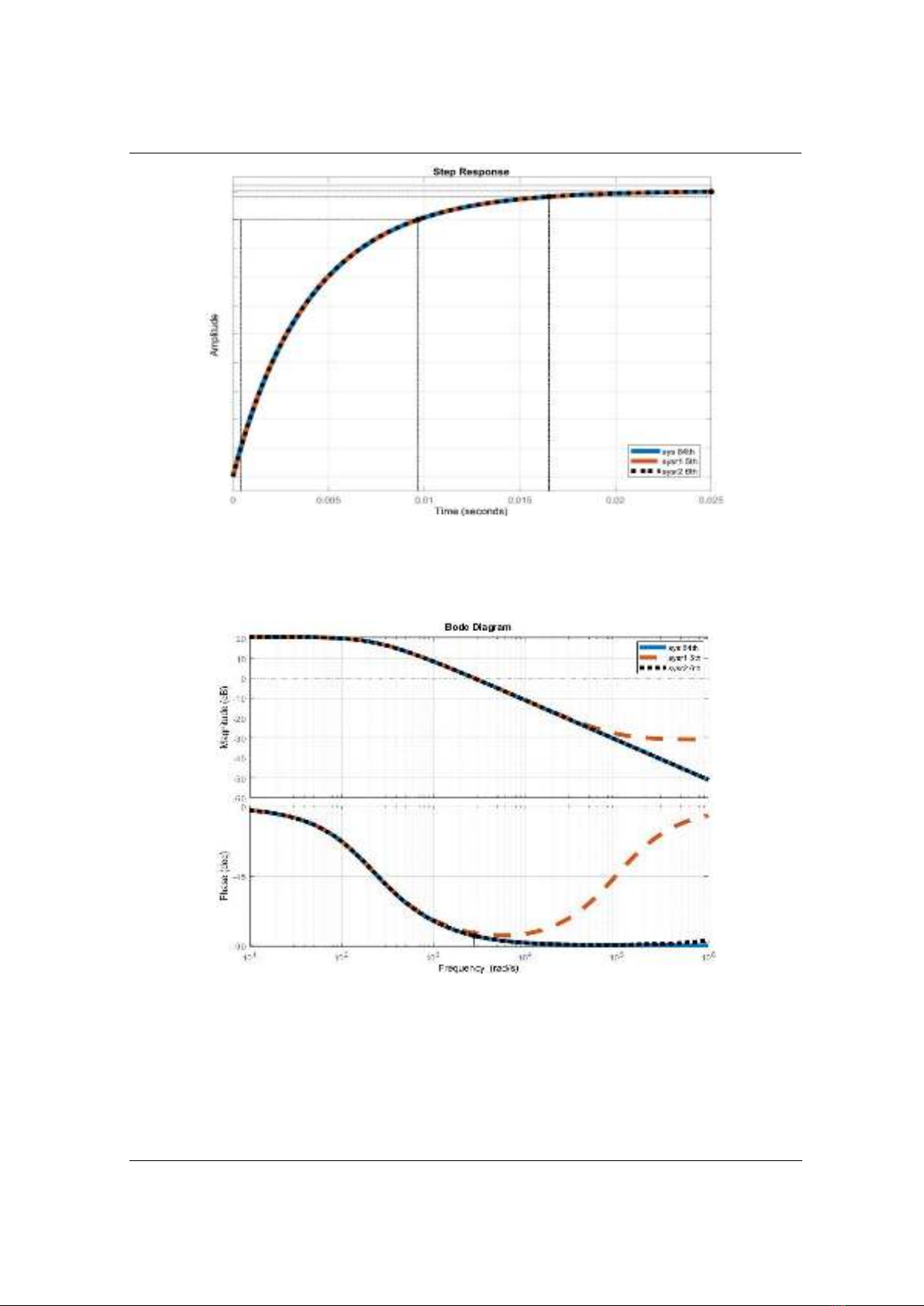
Figure 1. Impulse response Comparison between Reduced-Order Systems and the Original System
From Figure 1, it is observed that the 5th and 6th-order reduced-order systems exhibit transient
responses matching those of the original system. Hence, either the 5th or 6th-order reduced-order
system can be employed as a viable replacement for the original system in applications across the
time domain.
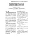
Figure 2. Frequency response Comparison between Reduced-Order Systems and the Original System
Figure 2 reveals that the 6th-order reduced-order system demonstrates a frequency domain
response that aligns with that of the original system. On the other hand, the 5th-order reduced-order
system exhibits a Magnitude response matching the original system at frequencies below 3x10⁴
(rad/s) (at 20 dB) and a Phase response matching the original system at frequencies below 2x10³
(rad/s) (at 80 deg). However, significant discrepancies are evident at higher frequency ranges.
Consequently:

TNU Journal of Science and Technology
229(06): 51 - 56
http://jst.tnu.edu.vn 55 Email: jst@tnu.edu.vn
- The 6th-order reduced-order system can be effectively employed as a substitute for the original
system across the entire frequency spectrum.
- The 5th-order reduced-order system can serve as a replacement for the original system in
applications involving Magnitude response at frequencies below 3x10⁴ (rad/s) and Phase response
at frequencies below 2x10³ (rad/s).
The order reduction system has the following state space model:
- The system reduces to order 5th:
11
323.2 217 15.49 40.73 5.681 53.13
215 840.3 27.95 18.25 165.9 0.1013
,
2.325 32.77 250.2 96.57 40.49 0.003456
42.63 23.93 94.26 299.9 238.6 0.1089
3.246 149.9 37.57 209.7 1193
sys sys
AB
11
, [ ]
0.06563
8.42 06
53.13 0.1039 0.008405 0.1131 0.0706
sys sys e
DC
- The system reduces to order 6th:
2
322 164.5 145.9 2.406 38.34 6.59
169.6 479.5 266.7 94.94 72.39 84.37
141.9 267 631.8 65.76 10.68 95.37
2.382 99.53 60.4 244.9 7.087 39.93
25.67 39.1 35.14 1.491 296.1 165.2
2.326 74.52 85.88 27.27 185.1 55
sys
A
7
2
22
53.13
0.02177
0.03364
,0.003578
0.01048
7.8 0.02778
53.13 0.0224 0.03342 0.004399 0.01651 0.02849 , 3.467 10
sys
sys sys
B
CD
The absolute and relative errors based on the H∞ norm between the original system and the 5th
and 6th-order reduced-order systems are presented in Table 1.
From Table 1, it is evident that the absolute error between the original system and the 5th-order
reduced-order system consistently exceeds that of the 6th-order reduced-order system. The absolute
error, as per the H∞ norm, indicates the maximum deviation between the original system and the
reduced-order system across the entire time domain, while the relative error, as per the H∞ norm,
signifies the greatest discrepancy between the original system and the reduced-order system across
the entire frequency spectrum.
Therefore, when accuracy is paramount, the BPRU algorithm appears to be the most effective
choice among these three algorithms for model reduction in this context.
Table 1. Comparison of Model Reduction Algorithms
Reduced Order (r)
Absolute Error
Relative Error
5
0.032286063250813
0.002979566832949
6
0.012067214855912
0.001113640671253
These results suggest that the 6th-order reduced-order system provides a more accurate
approximation of the original system, with significantly lower errors in both absolute and relative
terms. This information is crucial for understanding the trade-offs and selecting an appropriate
reduced-order model based on the desired accuracy for various applications across both time and
frequency domains.


![Tài liệu giảng dạy Vi tích phân A2 [chuẩn nhất]](https://cdn.tailieu.vn/images/document/thumbnail/2026/20260323/hoatudang2026/135x160/54651774420904.jpg)


![Tài liệu giảng dạy Hình học Affine và Euclide [chuẩn nhất]](https://cdn.tailieu.vn/images/document/thumbnail/2026/20260323/hoatudang2026/135x160/52531774414221.jpg)


