MEASURE Evaluation_3

Chia sẻ: Thao Thao | Ngày: | Loại File: PDF | Số trang:12

Thêm vào BST

Báo xấu

29
lượt xem 4
download

Download Vui lòng tải xuống để xem tài liệu đầy đủ

Tham khảo tài liệu 'measure evaluation_3', kỹ thuật - công nghệ, cơ khí - chế tạo máy phục vụ nhu cầu học tập, nghiên cứu và làm việc hiệu quả

Chủ đề:

Bình luận(0) Đăng nhập để gửi bình luận!

Lưu

Nội dung Text: MEASURE Evaluation_3

Simpo PDF Merge and Split Unregistered Version - http://www.simpopdf.com between the smallest and the largest value tionof the population contained size 10 - I 1 cation on 0 a samp e = 11 . e meanIng 0 t e qua IS 10 + 1 the average " should be properly understood. For any particular sample of size 10, the actual fraction of the population contained in the interval Z:: But if the average of those X(N) X(1) will generally not be equal to Z:: fractions is taken for many samples of size N, it will be close to Tolerance intervals involving confidence coefficients One can formulate more specific questions related to coverages by in- of the statement about troducing, in addition to the coverage, the confidence the coverage. For example, one can propose to find two order statistics such that the confidence is at least 90 percent that the fraction of the population contained between them (the coverage) is 95 percent. For a sample of size 200 , these turn out to be the third order statistic from the bottom and the third order statistic from the top (see Table A30 in Natrella ). For further discussion of this topic , several references are recommended. Non-normal distributions and tests of normality Reasons for the central role of the normal distribution in statistical theo- ry and practice have been given in the section on the normal distribution. Many situations are encountered in data analysis for which the normal distri- bution does not apply. Sometimes non-normality is evident from the nature of the problem. Thus , in situations in which it is desired to determine wheth- er a product conforms to a given standard , one often deals with a simple di- chotomy: the fraction of the lot that meets the requirements of the standard, and the fraction of the lot that does not meet these requirements. Tbe statisti- (see section on cal distribution pertinent to such a problem is the binomial the binomial distribution). In other situations, there is no a priori reason for non-normality, but the data themselves give indications of a non-normal underlying distribution. Thus, a problem of some importance is to " test for r.ormality. Tests of normality Tests of normality should never be performed on small samples , be- cause small samples are inherently incapable of revealing the nature of the underlying distribution. In some situations, a sufficient amount of evidence is gradually built up to detect non-normality and to reveal the general nature of the distribution. In other cases, it is sometimes possible to obtain a truly large sample (such as that shown in Table 4. 1) for which normality can be tested by " fitting a normal distribution " to the data and then testing the goodness of the fit."5 A graphical procedure for testing for normality can Probability plots. be performed using the order statistics of the sample. This test is facilitated through the use of " normal probability paper " a type of graph paper on which the vertical scale is an ordinary arithmetic scale and the horizontal
p. == p, p~ Simpo PDF Merge and Split Unregistered Version - http://www.simpopdf.com represent the fraction of individuals having the stated character- Let istic (serum glucose greater than 110 mg/dl) in the and let sample of size N; It is clear that for a relatively small , or even a moderately large =I- is a random variable with a well- In fact P. N, p will generally differ from binomial. defined distribution function, namely the can be shown to be equal The mean of the binomial (with parameter P) Thus to P. (4. 24) E(P) another name represents the " expected value " of where the symbol E(P) for the population mean. Thus the population mean of the distribution of will P. If equal to the parameter is taken as an estimate for this estimate unbiased. therefore be Furthermore: V ar(p) = (4. 25) Hence ( 4. 26) The normal approximation for the binomial distribution It is a can be remarkable fact that for a large the distribution of approximated by the normal distribution of the same mean and standard de- viation. This enables us to easily solve practical problems that arise in con- nection with the binomial. For example , returning to our sample of 100 indi- viduals from the population given in Table 4. , we have: ,. = 0. E(P) 785) (0, ~ 0, 0411 CT, i~, From these values = 100 from the , one may infer that in a sample of population in question values of less than 0. , the chance of obtaining (two standard deviations below the mean) or of more than 0. 30 (two standard deviations above the mean) is about 5 percent. In other words , the chances are approximately 95 percent that in a sample of 100 from the population in question the number of individuals found to have serum glucose of more than 110 mg/dl will be more than 13 and less than 30. Since , in practice is generally unknown, all inferences , the value of must then be drawn from the sample itself. Thus, if in a sample of 100 one finds ap value of, say, 0. 18 (i. , 18 individuals with glucose serum greater and con- than 110 mgldl), one will consider this value as an estimate for sequently one will take the value
Simpo PDF Merge and Split Unregistered Version - http://www.simpopdf.com (0. 18)(1 - 0. 18) = 0. 038 100 This would lead to the following approximate 95 per- as an estimate for cr P' cent confidence interval for 0.18 - (1.96)(. 038) .c P .c 0. 18 + (1.96)(. 038) .c 0. 10 .c The above discussion gives a general idea about the uses and usefulness of the binomial distribution. More detailed discussions will be found in two general references. Precision and accuracy The concept of control In some ways , a measuring process is analogous to a manufacturing process. The analogue to the raw product entering the manufacturing proc- ess is the system or sample to be measured. The outgoing final product ofthe manufacturing process corresponds to the numerical result produced by the also applies to both types ofproc- measuring process. The concept of control esses. In the manufacturing process , control must be exercised to reduce to minimum any random fluctuations in the conditions of the manufacturing , the equipment. Similarly, in a measuring process, one aims at reducing to a mini- mum any random fluctuations in the measuring apparatus and in the environ- mental conditions. In a manufacturing process , control leads to greater uni- formity of outgoing product. In a measuring process, control results in high- I.e. , in less random scatter in repeated measurements of the precision, er same quantity. Mass production of manufactured goods has led to the necessity of inter- changeability of manufactured parts, even when they originate from differ- ent plants. Similarly, the need to obtain the same numerical result for a par- ticular measurement , regardless of where and when the measurement was control of a measuring process is not enough. Users made, implies that Local control , aimed at assuring a high degree of " in- interlaboratory also require terchangeability " of results , even when results are obtained at different times or in different laboratories. Methods of monitoring a measuring process for the purpose of achiev- ing " local" (I.e. , within- laboratory) control will be discussed in the section on quality control of this chapter. In the following sections, we will be con- cerned with a different problem: estimating the precision and accuracy of a of measurement. method Within- and between- laboratory variability Consider the data in Table 4. 6, taken from a study of the hexokinase method for determining serum glucose. For simplicity of exposition, Table
..., ..., Simpo PDF Merge and Split Unregistered Version - http://www.simpopdf.com graduated in terms of labeled coverages scale is (from 0 to 100 percent), but in terms of the reduced z-values corresponding to these coverages (see sec- tion on the normal distribution). More specifically, suppose we divide the 1 segments such that the area abscissa of a plot of the normal curve into ' The under the curve between any two successive division points is the values of which can be determined division points will be Z2, ZN, curve. Table 4. 5 lists the from the normal values ~2'..., ' in percent , in column 1, and the values in corresponding normal 10. According to the general theorem about order statis- column 2, for = 10 " attempt" to accomplish tics, the order statistics of a sample of size 1 equal parts. Consequently, the just such a division of the area into values. The order statistics order statistics tend to be linearly related to the for the first sample of Table 4. 2 are listed in column 3 of Table 4. 5. A plot of column 3 versus column 2 will constitute a " test for normality : if the data are normally distributed , the plot will approximate a straight line. Further- more, the intercept of this line (see the section on straight line fitting) will be an estimate of the mean , and the slope of the line will be an estimate of the standard deviation. 2 For non-normal data , systematic departures from a straight line should be noted. The use of normal probability paper obviates the calculations involved in obtaining column 2 of Table 4. 5, since the hori- but labeled according to the values zontal axis is graduated according to , expressed as percent. Thus , in using the probability paper , the ten ~1 order statistics are plotted versus the numbers 100 100 100 - U' Tt ' or 9. 09, 18. 18, . . . , 90. 91 percent. It is only for illustrative purposes that we have presented the procedure by means of a sample of size 10. One would generally not attempt to u~e this method for samples of less than 30. Even then , subjective judgment is required to determine whether the points fall along a straight line. In a subsequent section , we will discuss transformations of scale as a means of achieving normality. The binomial distribution Referring to Table 4. , we may be interested in the fraction of the popu- lation for which the serum glucose is greater than , say, 110 mgldl. A problem of this type involves partitioning the range of values of a continuous variable (serum glucose in our illustration) into two groups , namely: (a) the group of individuals having serum glucose less than 110 mgldl; and (b) the group individuals having serum glucose greater than 11 0 mgldl. (Those having se- rum glucose exactly equal to 110 mgldl can be attached to one or the other group, or their number divided equally among them.
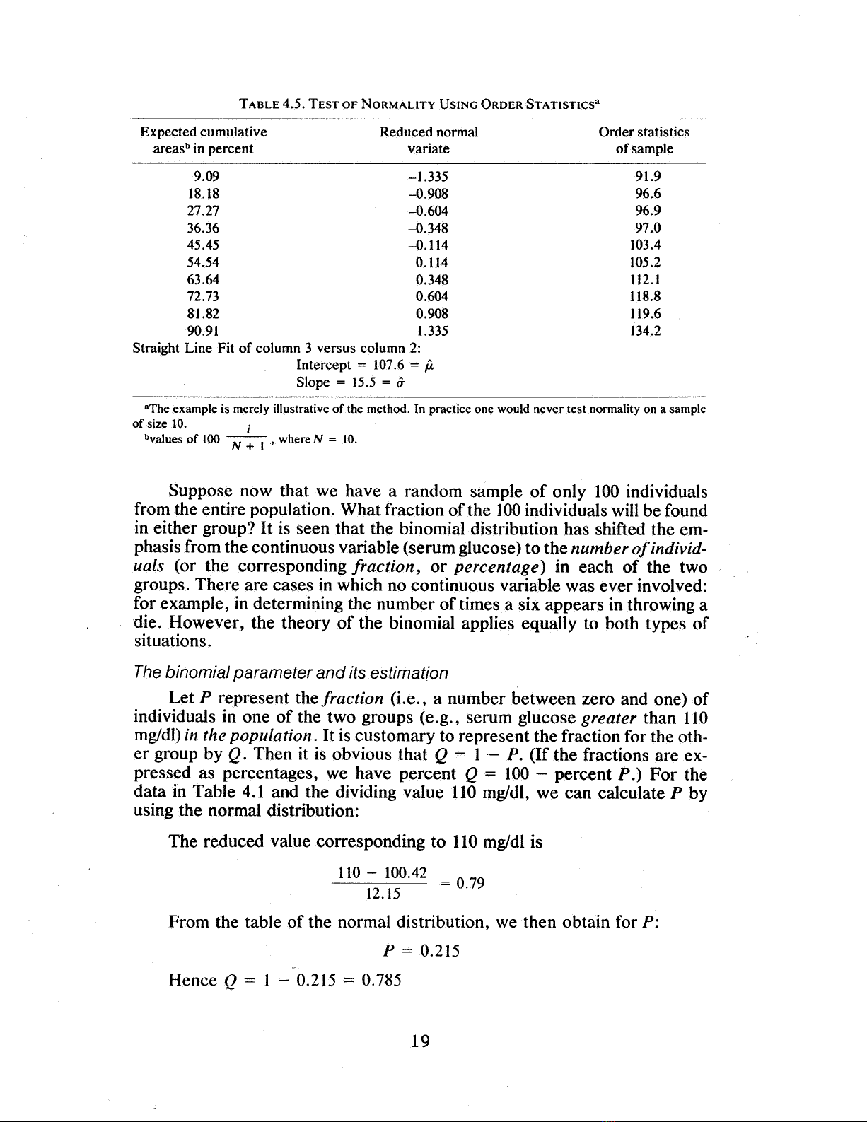
Simpo PDF Merge and Split Unregistered Version - http://www.simpopdf.com TABLE 4. 5. TEST OF NORMALITY USING ORDERSTATISTlCSa 09 -0. 18 - Order statistics Reduced normal Expected cumulative areas b in percent variate of sample 27 -0. 36 0. 91.9 1.335 45 96. 908 18. 54 96. 27. 604 64 -0.348 97. 36. 73 0. 45. 103.4 114 82 54. 105. 114 91 63. 348 112. 72. 604 118. 81. 908 119. 90. 1.335 134. Straight Line Fit of column 3 versus column 2: Intercept == 107. 6 = P- Slope = 15. 5 = a- aThe example is merely illustrative of the method. In practice one would never test normality on a sample of size 10. 10. values of 100 ' where +l Suppose now that we have a random sample of only 100 individuals from the entire population. What fraction of the 100 individuals will be found in either group? It is seen that the binomial distribution has shifted the em~ number of individ~ phasis from the continuous variable (serum glucose) to the in each of the two uals (or the corresponding or percentage) fraction, groups. There are cases in which no continuous variable was ever involved: for example, in determining the number of times a six appears in throwing a die. However, the theory of the binomial applies equally to both types of situations. The binomial parameter and its estimation (I.e. , a number between zero and one) of Let represent the fraction individuals in one of the two groups (e. than 110 greater , serum glucose It is customary to represent the fraction for the oth~ mgldl) in the population. (If the fractions are ex~ er group by Then it is obvious that P. 1 .- Q. For the pressed as percentages = 100 - , we have percent percent data in Table 4. 1 and the dividing value 110 mgldl , we can calculate using the normal distribution: The reduced value corresponding to 110 mgldl is 15 110 - 100.42 = 0 79 12. From the table of the normal distribution , we then obtain for = 0. 215 1 - 0. 215 == 0. 785 Hence
Simpo PDF Merge and Split Unregistered Version - http://www.simpopdf.com TABLE 4. 6. DETERMINATION OF SERUM GLUCOSE Serum sample Laboratory 40. 76. 206. 137. 42.3 78. 208.5 137.4 77. 42. 204. 138. 77. 40. 210. 138. 43.4 211.6 78. 135. 43. 76. 201.2 131.3 43. 76. 201.2 146. 42. 75. 133.4 208. 41.3 75. 205. 134. 40. 76. 200. 134. 40. 76. 206. 131.5 42. 76.4 133.4 199. BAli results are expressed in mg glucose/dl. 6 contains only a portion of the entire set of data obtained in this study. Each of three laboratories made four replicate determinations on each of four serum samples. It can be observed that, for each sample, the results laboratories tend to show greater differences than re- different obtained by sults obtained through replication in the same laboratory. This observation can be made quantitative by calculating, for each sample, two standard de- viations: the standard deviation " within " laboratories and the standard de- viation " between laboratories. Within- laboratory precision is often re- reproduc- and between- repeatability, ferred to as laboratory precision as ibility. We will illustrate the method for serum sample A. The data for serum A can first be summarized as follows: Laboratory A verage 41.500. 0. 2 43. 15 0. Standard Deviation 938 41.02 635 793 The three standard deviations could be averaged to obtain an " average within- Iaboratory standard deviation. However , if one can assume that these three standard deviations are estimates of one and the same population a better way is to " pool" the variances, 2 and take the standard deviation , square root of the pooled variance. Using this procedure, we obtain for the best estimate of the within- laboratory sw standard deviation 5~-;:-LO:i93i ~ 0. 798 (O. 8)' liQ. Let us now calculate the standard deviation among the three average values 41.50 43. we obtain: , and 41.02. Denoting this standard deviation by S:r,
-=- Simpo PDF Merge and Split Unregistered Version - http://www.simpopdf.com 1.117 s;r If the laboratories displayed no systematic differences, this standard devia- tion , being calculated from averages of four individual results , should be = 0. 798/V4 = 0. 399. The fact that the calculated value, equal to /V4 1.117, is appreciably larger than 0. 399 can be explained only through the presence of an additional between- component of variability. laboratory This component , expressed as a standard sL deviation and denoted by stands for " laboratories ), is calculated by subtracting the " antici- (where pated" variance, (0. 399)2 , from the " observed" variance, (1.117)2 , and tak- ing the square root: = v(LlI 7)2 = 1. (0.3 99)2 s(- The calculations for an four serum samples are summarized in Table 4. , in which standard deviations are rounded to two decimal places. It may be inferred from Table 4. tends to increase with the glu- 7 that sw shows cose content of the sample. The between- laboratory component, s L, no such trend. However , the data are insufficient to establish these facts with. reasonable confidence. Since our purpose is to discuss general prin- ciples , and the use of these data is only illustrative, we will ignore these shortcomings in the discussion that follows. Accuracy--comparison with reference values The two components of the method. To Sw SL, precision and define the for an samples. Let us accuracy, reference values estimate its one requires assume that such values have been established and are as fonows: . 76. 40. Serum Sample B Reference Value . D 204. 133.4 The values given here as " reference values " are actuany only tentative.. We will assume, however present discussion , that they can be considered , in our to be free of systematic errors. Our task is to decide whether the values ob- tained in our study are equal to these within random experimental error, reference values. The grand average value for sample A , 41.89 mgldl , which TABLE 4. 7. SUMMARY OF ANALYSIS FOR SERUM GLUCOSE DATA Standard deviation . Serum sample Average (mg/dl) (mg/dl) (mg/dl) S I. s u' 41.89 1.04 76. 1.05 136. 1.07 205.41 1.08
.+ Simpo PDF Merge and Split Unregistered Version - http://www.simpopdf.com involves 12 individual determinations and four we denote by the symbol laboratories. Its variance, therefore, can be estimated by the formula: 12 (0.80)2 (1.04)2 = 0. s:r Now differs from the reference value by the amount: 8 = 1.09 41.89 - 40. Corresponding values for all four samples are shown in Table 4. It can be seen that, on the one hand, all four grand averages are larger than the corresponding reference values but, on the other hand, the differ- One would s~. of ences are of the order only one or two standard errors tentatively conclude that the method shows a positive systematic error (bias) but , as has been pointed out above, the data are insufficient to arrive at defi- nite conclusions. Straight line fitting great im- of of The fitting straight lines to experimental data is a subject portance , particularly in analytical laboratories. Many analytical and clinical methods make extensive use of linear calibration curves for the purpose converting a measured quantity, such as an optical absorbance or a ratio peaks-heights on a mass-spectrometer scan , into a concentration value for an unknown constituent. Calibration curves are established by subjecting known concentrations to the measuring process and fitting lines samples of the measure- be the known concentration to the resulting data. Let , and ment (e. paired val- of , optical absorbance). The data will consist of a set ues, as shown for an illustrative and example in the columns labeled Table 4. the table shows that there is a " blank" : for zero concen Inspection of tration , one finds a nonzero absorbance value. If one " corrected" the sub- sequent two values for the blank , one would obtain 0. 189 - 0. 050 = 0. 139, and 0. 326 - 0. 050 == 0. 276. lethe " corrected" absorbance were proportion- al to concentration (as required by Beer s law), these two corrected absor- 1 to 2. Ac- bances should be proportional to 50 and 100 , I.e. of , in a ratio tually, 0. 139 is slightly larger than (0. 276/2). We will assume that this is due TABLE 4. 8. STUDY OF ACCURACY OF GLUCOSE DETERMINATION Serum sample Grand average Reference value (R) (1) 40. 41.89 1.09 76. 76. 0.41 133.4 136. 1.29 204. 205.41 1.25 1.31
y= " = === y= .. Simpo PDF Merge and Split Unregistered Version - http://www.simpopdf.com TABLE 4. 9. CALIBRATION CURVE FOR GLUCOSE IN SERUM 050 0516 0016 189 0005 1895 326 100 3273 0013 0.467 150 0.4652 0015 200 605 6030 0020 400 1.156 1.1545 0015 600 I. 704 1.7059 0019 214. 6425 6425 0516 + 0. 0027571 x . = 0. 0019 glucose, in mg/dl x = concentration of absorbance fitted value residual d= solely to experimental error in the measured absorbance values, thus assum- ing that any errors in the concentration values are negligibly -small. general model If a represents the true value of the " blank" and 13 the absorbance per unit concentration , we have, according to Beer s law: (4. 27) E(y) . ~ a = f3x where E(y) is the expected value for absorbance, I.e. , the absorbance value freed of experimental error. Now the actual absorbance, y. is affected by an experimental error Hence: , which we will denote bye. (4. 28) y = E(y) + e + e (4. Combining Equations 4. 27 and 4. 28 we obtain the " model" equation 29) a+ f3x This equation- with the same Le. should hold for all x-values, xt.x2, XlV. values of a and 13. Hence + ei (4. 30) Yi = a + f3Xi where i= 1 to N. The errors ei should, on the average, be zero, but each one departs from zero by a random amount. We will assume that these random departures from zero do not increase with the absorbance (in some cases, this assumption is not valid) and that their distribution is Gaussian with standard deviation 0" P' The object of the analysis is to estimate: (a) a and 13, as well as the uncer- tainties (standard errors) of these estimates; and (b) the standard deviation of e; i.e. O"e.
Simpo PDF Merge and Split Unregistered Version - http://www.simpopdf.com Formulas for linear regression The fitting process is known in the statistical literature as the " linear 13, (T e by x. We will denote the estimates of on /3, and regression of respectively. The formulas involve the following three quantities: and S e, U= (4.31) i)2 I(Xi (4. 32) = I(Yi - ji)2 (4.33) - i)(Yi - ji) I(Xi In terms of these three quantities, we have the formulas: a=y- j3i (4. 34) /3 = (JnjU) (4.35) N- vV (4. 36) Se I Sa Sp For the data of Table 4. 9, the calculations result in the following values: = 0. 0000036 Se = 0. 0019. = 0. 0010 13 = 0. 0027571, = 0. 0516, sa Sa a " calcu- and 13 are x, now available, we can calculate, for each Since This is , of lated" (or " fitted" ) value, y, given by the equation 13x. course, simply the ordinate of the point on the fitted line for the chosen value ofx. and the calculated value y The differences between the observed value residual." Table 4. 9 also contains the values of y and the resid- is called a " uals, denoted by the symbol" occurring in It is important to observe that the P2/U), (W quantity Thus: Equation 4. 35. Id~. , is simply equal to ~d' (4.37) N~ This formula, though mathematically equivalent to Equation 4.35, should be used in preference to Equation 4.35, unless all calculations are carried out are di with many significant figures. The reason for this is that the quantities P2/U). (W less affected by rounding errors than the quantity residua/s-weighting of Examination The residuals should behave like a set of random observations with a It follows that the algebraic signs and a standard deviation (J" e' mean of zero should exhibit a random pattern similar to the occurrence of heads and tails in the flipping of a coin. In our example, the succession of signs raises some suspicion of nonrandom ness, but the series is too short to decide on this mat- small , and the ter one way or the other. In any case, the errors are quite calibration curve is quite satisfactory for the intended purpose.
= - ~- = Simpo PDF Merge and Split Unregistered Version - http://www.simpopdf.com The assumptions underlying this procedure of fitting a straight line are i have the not always fulfilled. The assumption of homoscedasticity (I.e., all same standard deviation), in particular, is often violated. If the standard de- the fitting of the Xi' ei is nonconstant and depends on viation of the error weighted regression analysis. straight line requires the application of " one defines a " weight" i, for each (Fe. Briefly, assuming a different value of (Fe. Thus: equal to the reciprocal of the square l of Wi (4.38) = l/(F W' are then used in the regression calculations , leading to for- Wi The weights mulas that are somewhat different from those given in this section. For fur- ther details, two references can be consulted. Propagation of errors It is often necessary to evaluate the uncertainty of a quantity that is not directly measured but is derived, by means of a mathematical formula, from directly measured. are other quantities that An example As an example, consider the determination of glucose in serum, using an enzymatic reaction sequence. The sequence generates a product, the opti- cal absorbance of which is measured on a spectrophotometer. The proce- dure consists of three steps: (a) apply the enzyme reaction sequence to a set of glucose solutions of known concentrations, and establish in this way a cal- ibration curve of " absorbance " versus " glucose concentration " (b) by use measure the absorbance for the " un- of the same reaction sequences, known, " and (c) using the calibration curve, convert the absorbance for the unknown into a glucose concentration. It turns out that the calibration curve, for this sequence of reactions, is concentration, the calibration Thus , ify represents absorbance , and linear. cu!'ve is represented by the equation: y=a+f3x (4. 39) val- The calibration curve is established by measuring y for a set of known ues. We will again use the data of Table 4. 9 for illustration. Fitting a straight line to these data , we obtain: y = 0. 0516 + 0. OO27571x (4.40) times Let us now suppose that an unknown sample of serum is analyzed = 0. 3672 = 4), and that the average absorbance found is Yu (for example, stands for absorbance for the unknown). Using the calibration (where Yu by solving the Xu, into a concentration value, line, we convert the value Yu calibration equation for 0.3672 - 0. 0516 YIl (4 AI) o.OO27571 = 114.47 mgldl XI) How reliable is this estimate?
) + (- + . . . )+... .., ..., .... )+ Simpo PDF Merge and Split Unregistered Version - http://www.simpopdf.com Let us assume, at this point , that the uncertainty of the calibration line and it is readily is negligible. Then the only quantity affected by error is Yu, is equal to that ofyu, divided by seen from Equation 4.41 that the error of Xu If we assume that the standard deviation of a single measured y-value is 13. the average of four 0019 absorbance units , then the standard error of Yu, determinations , is v4 = 0. 00095 0019/ Xu Hence the standard deviation of 00095/13 = 0. 00095/0. 0027571 = 0. 34 mg/dl A more rigorous treatment would also take account of the uncertainty of the calibration line. The general case can be a function of several More generally, a calculated quantity each of which is affe.cted by experimen- measured quantities Xb Xz, X3, tal error. The problem to be solved is the calculation of the standard devia- as a function of the standard deviations of the errors of tion of the error of X.. Xz, X3, errors in the quantities independent We will only deal with the case of , we assume that the error s is totally . . . ; i.e. Xz, X3, of any one of the For independent errors in the meas- s. unaffected by the errors in the other some simple rules can be applied. They . are all ured values x.. Xz, X3,' derived from the application of a general formula known as " the law of prop- agation of errors " which is valid under very general conditions. The reader is referred to Mandelz for a general discussion qf this formula. Linear relations. For (4.42) Xl azxz x3 the law states: Var(xl ) (4.43) Var(x3 + ai Var(xz ai a~ Var(y) = As an example, suppose that the weight of a sample for chemical analysis has been obtained as the difference between two weights: the weight of an and the weight of the crucible containing the sample, empty . Wi, crucible, is equal to Wz. Thus the sample weight (4.44) - Wl Wz S=t This is in accordance with Equation 4.42 by writing: 1)Wz (1)Wl Hence , according to Equation 4.43 I)2Var(W2 Var(S) = (l)2Var(Wl Var(S) = Var(Wl ) + Var(W2