Hence
(J"s = v' 0-2w, 0-2W2 (4.45)
Note that in spite of the negative sign occurring in Equation 4.44, the vari-
ances of WI and W 2 in Equation 4.45 are added (not subtracted from each
other).
It is also of great importance to emphasize that Equation 4.43 is valid
only if the errors in the measurements Xh X2, Xa, . . . , are independent
each other. Thus, if a particular element in chemical analysis was deter-
mined as the difference between 100 percent and the sum of the concentra-
tions found for all other elements, the error in the concentrations for that
element would not be independent of the errors of the other elements, and
Equation 4.43 could not be used for any linear combination of the type of
Equation 4.42 involving the element in question and the other elements. But
in that case, Equations 4.42 and 4.43 cou\d be used to evaluate the error vari-
ance for the element in question by considering it as the dependent variable
y.
Thus, in the case of three other elements Xl' X2, and Xa, we would have:
= 100 - (Xl + X2 + xa
where the errors of X2, and Xa are independent. Hence:
Var(y) = Var(xI) + Var(x2) + Var(xa
since the constant, 100 , has zero-variance.
Products and ratios. For products and ratios, the law of propagation
of errors states that the squares of the coefficients of variation are additive.
Here again, independence of the errors is a necessary requirement for the
validity of this statement. Thus, for
= Xl .
with independent errors for I and X2, we have.
(4.46)
(100 :u
= (100
::'
r + (100
::2
We can, of course , divide both sides of Equation 4.47 by 1002, obtaining:
(4.47)
:u
= ( ::'
r + (
::2 (4.48)
Equation 4.48 states that for products of independent errors, the squares of
the relative errors are additive.
The same law applies for ratios of quantities with independent errors.
Thus, when Xl and X2 have independent .errors , and
y=-
(4.49)
we have
r = (
::'
r + (
::2 (4. 50)
Simpo PDF Merge and Split Unregistered Version - http://www.simpopdf.com
As an illustration, suppose that in a gravimetric analysis , the sample weight
is S, the weight of the precipitate is and the " conversion factor" is
Then:
= 10OF
The constants 100 and are known without error. Hence, for this example,
r +(
, for example, the coefficient of variation for is 0. 1 percent, and that for
is 0. 5 percent, we have:
= V (0.005)2 + (0. 001)2 = 0.0051
It is seen that in this case , the error of the sample weight has a negligible
effect on the error of the "unknown
Logarithmic functions. When the calculated quantity is the natural
logarithm of the measured quantity (we assumed that 0):
= In
the law of propagation of error states
(4. 51)
(Tx
(T (4. 52)
For logarithms to the base 10, a multiplier must be used: for
loglo
the law of propagation of error states:
(4.53)
-;-
(4. 54)
Sample sizes arid compliance with standards
Once the repeatability and reproducibility of a method of measurement
are known, it is a relatively simple matter to estimate the size of a statistical
sample that will be required to detect a desired effect, or to determine wheth~
er a given specification has been met.
An example
As an illustration , suppose that a standard requires that the mercury
content of natural water should not exceed 2J.Lgll. Suppose, furthermore
that the standard deviation of reproducibility of the test method (see section
on precision and accuracy, and MandeF), at the level of 2J.Lgll is 88J.Lgll.
subsamples of the water sample are sent to a number of laboratories and
Simpo PDF Merge and Split Unregistered Version - http://www.simpopdf.com
each laboratory performs a single determination, we may wish to determine
the number of laboratories that should perform this test to ensure that we
can detect noncompliance with the standard. Formulated in this way, the
problem has no definite solution. In the first place , it is impossible to guaran-
tee unqualifiedly the detection of any noncompliance. After all, the decision
will be made on the basis of measurements, and measurements are subject to
experimental error. Even assuming, as we do, that the method is unbiased,
we still have to contend with random errors. Second , we have, so far, failed
to give precise meanings to the terms "compliance " and " noncompliance
while the measurement in one laboratory might give a value less than 2,ugll
of mercury, a second laboratory might report a value greater than 2,ug/l.
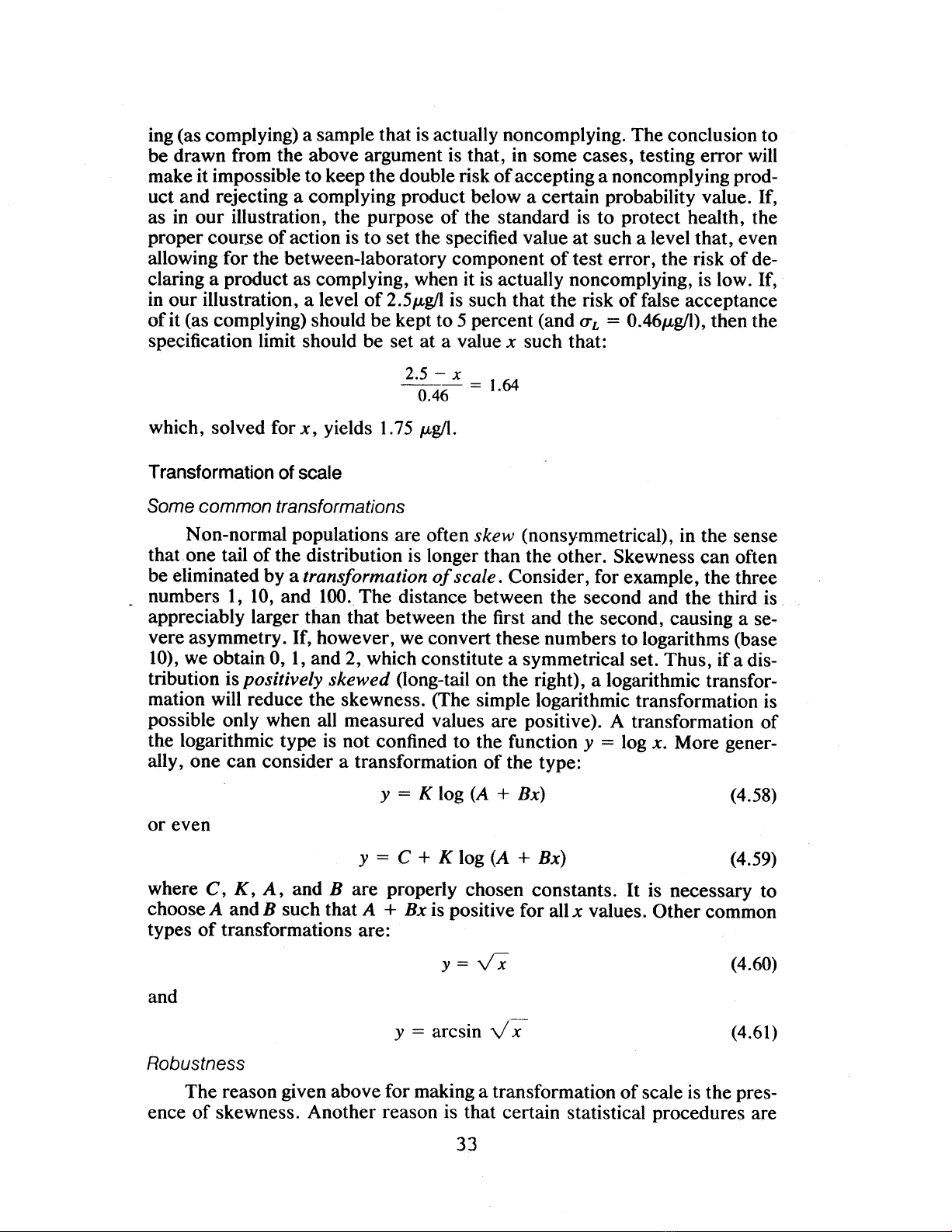
General procedure-acceptance, rejection, risks
To remove all ambiguities regarding sample size, we might proceed in
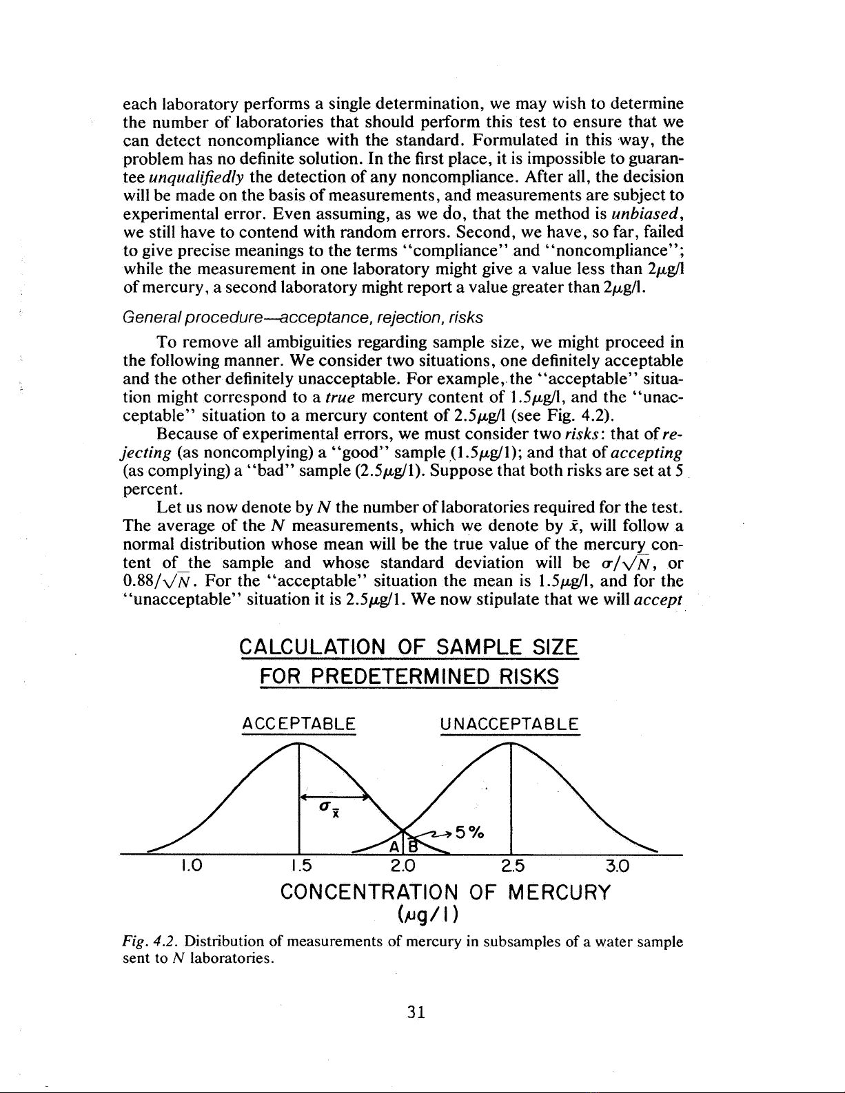
the following manner. We consider two situations, one definitely acceptable
and the other definitely unacceptable. For example,. the
' '
acceptable" situa-
tion might correspond to a true mercury content of 1.5,ugll, and the "unac-
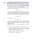
ceptable" situation to a mercury content of 5,ugll (see Fig. 4. 2).
Because of experimental errors, we must consider two risks: that of re-
jecting (as noncomplying) a "good" sample J1.5,ugll); and that of accepting
(as complying) a "bad" sample (2. 5,ugll). Suppose that both risks are set at 5
percent.
Let us now denote by the number of laboratories required for the test.
The average of the measurements, which we denote by i , will follow a
normal distribution whose mean will be the true value of the mercury con-
tent of the sample and whose standard deviation will be CT/
88/ . For the "acceptable" situation the mean is 1.5,ugll , and for the
unacceptable" situation it is 5,ugll. We now stipulate that we will accept
CALCULATION OF SAMPLE SIZE
FOR PREDETERMINED RISKS
ACCEPTABLE UNACCEPTABLE
0'
5 . 0 2..5 3.
CONCENTRATION OF MERCURY
(,ug/ I)
Fig. 4.2. Distribution of measurements of mercury in subsamples of a water sample
sent to laboratories.
Simpo PDF Merge and Split Unregistered Version - http://www.simpopdf.com
the sample, as complying, whenever is less than 2. , and reject , as non-
complying, whenever is greater than 2.0. As a result of setting our risks at
5 percent, this implies that the areas andB are each equal to 5 percent (see
Fig. 4. 2). From the table of the normal distribution, we read that for a 5 per-
cent one-tailed area, the value of the reduced variate is 1.64. Hence:
0 - 1.5
z = O. 88/
(We could also state the requirement that (2.0 - 2. 5)j(0.88j ) = ~ 1.64
which is algebraically equivalent to the one above.) Solving for N, we find:
= (
r = 8.
(4. 55)
We conclude that nine laboratories are required to satisfy our requirements.
The general formula, for equal risks of accepting a noncomplying sample and
rejecting a complying one, is:
= (
~ CT (4. 56)
where fT is the appropriate standard deviation, Zc is the value of the reduced
normal variate corresponding to the .risk probability (5 percent in the above
example), and is the departure (from the specified value) to which the cho-
senrisk probability applies.
Inclusion of between-laboratory variability
If the decision as to whether the sample size meets the requirements of a
standard must be made in a single laboratory, we must make our calculations
in terms of a different standard deviation. The proper standard deviation , for
an average of determinations in a single laboratory, would then be given
~:
u~ + u', (4.57)
The term a-Z must be included, since the laboratory mean may differ
from the true value by a quantity whose standard deviation is fTL' Since the
between-laboratory component ul is not divided by N, fT cannot be less
than (h no matter how many determinations are made in the single laborato-
ry. Therefore, the risks of false acceptance or false rejection of the sample
cannot be chosen at will. If in our case, for example, we had fTw == 0. 75J.tgll
and fTL -= 0.46J.Lg/I , the total fT cannot be less than 0.46. Considering the fa-
vorable case, J.L -= 1. 5J.Lg/I , the reduced variate (see Fig. 4.2) is:
0 - 1.5
46~"~ = 1.
This corresponds to a risk of 13. 8 percent of rejecting (as noncomplying) a
sample that is actually complying. This is also the risk probability of accept-
Simpo PDF Merge and Split Unregistered Version - http://www.simpopdf.com
ing (as complying) a sample that is actually noncomplying. The conclusion to
be drawn from the above argument is that, in some cases, testing error will
make it impossible to keep the double risk of accepting a noncomplying prod-
uct and rejecting a complying product below a certain probability value. If
as in our illustration , the purpose of the standard is to protect health , the
proper course of action is to set the specified value at such a level that, even
allowing for the between-laboratory component of test error, the risk of de-
claring a product as complying, when it is actually noncomplying, is low. If
in our illustration, a level of 5J..tg/l is such that the risk of false acceptance
of it (as complying) should be kept to 5 percent (and (h ;:: 0.46J..tg/1), then the
specification limit should be set at a value such that:
= t.
which , solved for yields 1.75 1Lg/1.
Transformation of scale
Some common transformations
Non-normal populations are often skew (nonsymmetrical), in the sense
that one tail of the distribution is longer than the other. Skewness can often
be eliminated by a transformation of scale. Consider, for example, the three
. numbers 1, 10, and 100. The distance between the second and the third is
appreciably larger than that between the first and the second, causing a se-
vere asymmetry. If, however, we convert these numbers to logarithms (base
10), we obtain 0 , 1 , and 2 , which constitute a symmetrical set. Thus, if a dis-
tribution is positively skewed (long-tail on the right), a logarithmic transfor-
mation will reduce the skewness. (The simple logarithmic transformation is
possible only when all measured values are positive). A transformation of
the logarithmic type is not confined to the function y ;:: log x. More gener-
ally, one can consider a transformation of the type:
y ;::
log (A Bx) (4. 58)
or even
;:: C + log (A Bx) (4. 59)
where C, K, A and are properly chosen constants. It is necessary to
choose and such that Bx is positive for all values. Other common
types of transformations are:
y= vx (4.60)
and
y ;:: arcsin (4.61)
Robustness
The reason given above for making a transformation of scale is the pres-
ence of skewness. Another reason is that certain statistical procedures are
Simpo PDF Merge and Split Unregistered Version - http://www.simpopdf.com
![Bảng tra dung sai lắp ghép Lê Hoàng Lâm: [Thêm từ mô tả phù hợp]](https://cdn.tailieu.vn/images/document/thumbnail/2022/20221205/camtucau205/135x160/9731670233749.jpg)


![Cẩm nang Gia công kim loại Việt Nam [mới nhất]](https://cdn.tailieu.vn/images/document/thumbnail/2026/20260513/baobinh_011/135x160/7971778670576.jpg)


![Giáo trình Hàn ống nâng cao (Nghề Hàn - CĐ) Trường Cao đẳng nghề Hải Dương [Mới nhất]](https://cdn.tailieu.vn/images/document/thumbnail/2025/20251212/laphong0906/135x160/47521779076565.jpg)


%20--%3e%3cdefs%3e%3cstyle%3e%20.st0%20{%20fill:%20%23fff;%20}%20.st1%20{%20fill:%20%237800fa;%20}%20%3c/style%3e%3c/defs%3e%3cpath%20class='st1'%20d='M117.78,12.18H43.11c2.9,3.47,4.65,7.94,4.65,12.82,0,5.6-2.3,10.66-6.01,14.29h76.02l7.22-13.56-7.22-13.56Z'/%3e%3cg%3e%3cpath%20class='st0'%20d='M53.58,26.17h-.59v-1.46h.59v-4.96h2.83c1.78,0,2.67.94,2.67,2.82v5.76c0,1.87-.89,2.81-2.67,2.81h-2.83v-4.96ZM55.36,21.37v3.34h1.1v1.46h-1.1v3.34h1.01c.61,0,.91-.37.91-1.1v-5.93c0-.74-.3-1.1-.91-1.1h-1.01Z'/%3e%3cpath%20class='st0'%20d='M65.99,31.14h-1.8l-.31-2.07h-2.19l-.31,2.07h-1.64l1.82-11.39h2.62l1.82,11.39ZM65.28,18.04c-.25.46-.51.77-.75.94-.21.15-.47.22-.79.22-.26,0-.57-.07-.92-.22l-.38-.15c-.14-.05-.26-.07-.37-.07-.3,0-.53.18-.71.54l-.91-.68c.25-.46.51-.77.75-.94.21-.14.48-.21.79-.21.26,0,.57.07.92.21l.38.15c.14.05.26.07.37.07.3,0,.53-.18.71-.54l.91.68ZM61.91,27.52h1.73l-.87-5.76-.87,5.76Z'/%3e%3cpath%20class='st0'%20d='M74.53,26.89v1.52c0,1.91-.89,2.86-2.67,2.86s-2.67-.95-2.67-2.86v-5.93c0-1.91.89-2.86,2.67-2.86s2.67.95,2.67,2.86v1.11h-1.69v-1.22c0-.75-.31-1.12-.93-1.12s-.93.37-.93,1.12v6.15c0,.74.31,1.11.93,1.11s.93-.37.93-1.11v-1.63h1.69Z'/%3e%3cpath%20class='st0'%20d='M81.4,31.14h-1.8l-.31-2.07h-2.19l-.31,2.07h-1.64l1.82-11.39h2.62l1.82,11.39ZM75.9,19.2l1.52-1.91h1.71l1.51,1.91h-1.61l-.76-.95-.75.95h-1.61ZM77.32,27.52h1.73l-.87-5.76-.87,5.76ZM83.1,15.99l-1.76,1.91h-1.26l1.17-1.91h1.86Z'/%3e%3cpath%20class='st0'%20d='M84.86,19.75c1.78,0,2.67.94,2.67,2.82v1.48c0,1.87-.89,2.81-2.67,2.81h-.85v4.28h-1.79v-11.39h2.64ZM84.01,21.37v3.86h.85c.58,0,.87-.36.87-1.08v-1.71c0-.71-.29-1.07-.87-1.07h-.85Z'/%3e%3cpath%20class='st0'%20d='M93.51,19.75c1.78,0,2.67.94,2.67,2.82v1.48c0,1.87-.89,2.81-2.67,2.81h-.85v4.28h-1.79v-11.39h2.64ZM92.66,21.37v3.86h.85c.58,0,.87-.36.87-1.08v-1.71c0-.71-.29-1.07-.87-1.07h-.85Z'/%3e%3cpath%20class='st0'%20d='M98.8,31.14h-1.79v-11.39h1.79v4.88h2.03v-4.88h1.83v11.39h-1.83v-4.88h-2.03v4.88Z'/%3e%3cpath%20class='st0'%20d='M105.36,24.55h2.46v1.62h-2.46v3.34h3.09v1.63h-4.88v-11.39h4.88v1.63h-3.09v3.18ZM108.17,17.29l-1.76,1.91h-1.26l1.17-1.91h1.86Z'/%3e%3cpath%20class='st0'%20d='M112.2,19.75c1.78,0,2.67.94,2.67,2.82v1.48c0,1.87-.89,2.81-2.67,2.81h-.85v4.28h-1.79v-11.39h2.64ZM111.35,21.37v3.86h.85c.58,0,.87-.36.87-1.08v-1.71c0-.71-.29-1.07-.87-1.07h-.85Z'/%3e%3c/g%3e%3ccircle%20class='st1'%20cx='25'%20cy='25'%20r='20'/%3e%3cpath%20class='st0'%20d='M32.78,19.27c2.92,0,4.43,2.55,5.28,5.33l.71,2.17c.14.38-.33.75-.71.75h-5.61c.19-.33.24-.71.09-1.08l-.75-2.45c-.43-1.32-.99-2.64-1.79-3.77.75-.57,1.65-.94,2.78-.94h0ZM25,18.38c3.25,0,4.9,2.78,5.89,5.89l.76,2.45c.14.42-.33.8-.8.8h-11.69c-.42,0-.94-.38-.8-.8l.75-2.45c.99-3.11,2.64-5.89,5.89-5.89h0ZM25,11.35c1.74,0,3.11,1.37,3.11,3.11s-1.37,3.11-3.11,3.11-3.11-1.41-3.11-3.11,1.41-3.11,3.11-3.11h0ZM17.27,19.27c1.08,0,1.98.38,2.73.94-.8,1.13-1.37,2.45-1.74,3.77l-.8,2.45c-.14.38-.05.75.09,1.08h-5.56c-.42,0-.9-.38-.75-.75l.71-2.17c.9-2.78,2.41-5.33,5.33-5.33h0ZM17.27,12.91c1.51,0,2.78,1.27,2.78,2.83s-1.27,2.83-2.78,2.83-2.83-1.27-2.83-2.83,1.27-2.83,2.83-2.83h0ZM32.78,12.91c1.56,0,2.78,1.27,2.78,2.83s-1.23,2.83-2.78,2.83-2.83-1.27-2.83-2.83,1.27-2.83,2.83-2.83h0ZM27.07,28.56v.09c0,.57-.24,1.08-.61,1.46h0v.05c-.38.33-.9.57-1.46.57s-1.08-.24-1.46-.61h0c-.38-.38-.61-.9-.61-1.46v-.09h1.41v.09c0,.19.05.38.19.47v.05c.09.09.28.19.47.19s.38-.09.47-.19v-.05c.14-.09.24-.28.24-.47t-.05-.09h1.41ZM30.99,28.56v.09c0,1.65-.66,3.16-1.74,4.24-1.08,1.08-2.59,1.79-4.24,1.79s-3.16-.71-4.24-1.79l-.05-.05c-1.04-1.08-1.7-2.55-1.7-4.2v-.09h1.41v.09c0,1.27.47,2.4,1.27,3.25h.05c.85.85,1.98,1.37,3.25,1.37s2.4-.52,3.25-1.37c.85-.8,1.37-1.98,1.37-3.25v-.09h1.37ZM34.99,28.56v.09c0,2.78-1.13,5.28-2.92,7.07-1.79,1.79-4.29,2.92-7.07,2.92s-5.23-1.13-7.07-2.92c-1.79-1.79-2.92-4.29-2.92-7.07v-.09h1.41v.09c0,2.4.94,4.53,2.5,6.08,1.56,1.56,3.72,2.5,6.08,2.5s4.52-.94,6.08-2.5c1.56-1.56,2.5-3.68,2.5-6.08v-.09h1.41Z'/%3e%3c/svg%3e)