
* Corresponding author.
E-mail addresses: arekhosravi@yahoo.com (A. Khosravi)
© 2013 Growing Science Ltd. All rights reserved.
doi: 10.5267/j.esm.2014.2.002
Engineering Solid Mechanics 2 (2014) 91-100
Contents lists available at GrowingScience
Engineering Solid Mechanics
homepage: www.GrowingScience.com/esm
Numerical method to measure velocity integration, stroke volume and cardiac
output while rest: using 2D fluid-solid interaction model
Arezoo Khosravia*, Hamidreza Ghasemi Bahrasemanb, Kamran Hassanib, and Davood Kazemi-Saleha
aAtherosclerosis research center, Baqiyatallah University of Medical Sciences, Tehran, Iran
bDepartment of Biomechanics, Science and Research Branch, Islamic Azad University, Tehran, Iran
A R T I C L E I N F O A B S T R A C T
Article history:
Received September 20, 2013
Received in Revised form
October, 14, 2013
Accepted 9 February 2014
Available online
12 February 2014
Development of knowledge of cardiovascular diseases and treatments strongly depends on
understanding of hemodynamic measurements. Hemodynamic parameters, therefore, have been
investigated using simulation-based methods. A two-dimensional model was applied for seven
healthy subjects with echo-Doppler at rest. Echocardiography imaging was also utilized to gain
the geometry of the aortic valve. Fluid-Structure Interaction (FSI) model was carried out,
coupling an Arbitrary Lagrangian-Eulerian mesh. Pressure loads were used as boundary
conditions on the valve’s ventricular and aortic sides. Pressure loads used were the calculated
brachial pressures plus differences between brachial, central and left ventricular pressures. The
FSI model predicted the velocity integration, stroke volume and cardiac output over a range of
heart rates while rest. Numerical results generally had a difference of 5.4 to 15.87% with
Doppler results. Linear correlations between numerical and clinical approaches have been
applied. This makes possible predictions achieved from the FSI model to be gained which are
highly accurate (e.g. correlation factor r = 0.995, 0.990 and 0.990 for velocity integration,
stroke volume and cardiac output, respectively). The obtained numerical results showed that
numerical methods can be combined with clinical measurements to provide good estimates of
patient specific hemodynamics for different subjects.
© 201
4
Growing Science Ltd. All rights reserved.
Keywords:
Echo-Doppler flow
Fluid-structure interaction
Hemodynamics
Natural aortic valve
1. Introduction
Disease of the heart and blood vessels is a major factor of mortality (Murphy & Xu, 2012). To
magnify the impact of recent methods applied to study the cardiovascular performance, it is crucial
that they are applied in clinically relevant researches. Comprehending changes to blood flow is a
fundamental element in cardiovascular diagnosis (Bodnar et al., 1999; Butchart et al., 2003; Criner et
al., 2010; Giddens et al., 1993). For example, such understanding may be used to evaluate patients
with coronary artery disease (Piérard & Lancellotti, 2007). Present invasive/non-invasive methods,

92
moreover, used to evaluate cardiovascular function have several restrictions, such as being arduous
and precious to use, as well as not being hazard free (Laske et al., 1996). Instead, mathematical
methods could be used to determine hemodynamics in addition to reducing the need for invasive
procedures.
Numerical methods have the possibility to estimate hemodynamics, only if the accurate boundary
conditions are used. Fluid-Structure Interaction (FSI) technique is pretty well suited to heart valve
simulations, like the aortic valve. Fluid flow around a valve causes its deflexion and deformation and
regulates valve opening and prepare it for closure (Pedley et al., 1978). Such recirculation depends on
the valve cusps deformation (Bellhouse, 1972). FSI simulations integrate Finite Element Analysis of
a solid with Computational Fluid Dynamics to evaluate flow. FSI uses of an Arbitrary-Lagrange-
Euler mesh to analyze the coupled physics (Donea et al., 1982; Formaggia & Nobile, 1999). A
concurrent FSI simulation could be applicable by constraints at boundaries which are shared by both
the structure and fluid. The reaction force of fluid exerts on the structure at the shared boundary,
while fluid velocity is restricted to be equal to the structural temporal deformation (Dowell & Hall,
2001; Van de Vosse et al., 2003).
FSI method has been used to examine biological (Al-Atabi et al., 2010; Espino et al., 2012a,b,c)
and artificial (Piérard & Lancellotti, 2007, Winslow, 1966) heart valves. The aortic valve, for
example, has been modelled in two- dimensions (De Hart et al., 2000) and three-dimensions (De Hart
et al., 2003a) as well as its leaflets have been considered as fiber-reinforced composites (De Hart et
al., 2003b). Griffith and Peskin (2005) and Griffith et al. (2007, 2009) provided a research included
an immersed boundary procedure for computational analysis of fluid-structure interaction of flexible
aortic valve for rest stage. Several aortic valve FSI simulations validated experimentally (De Hart et
al., 2000, 2003; Labrosse et al., 2010; Nobili et al., 2008). Such researches confirm the possibility of
developing complex aortic valve dynamics. However, up to now they have not been integrated with
non-invasive clinical computations to estimate a patient’s cardiac hemodynamics. Alterations to such
evaluation have not numerically been analysed either for several subjects.
The aim of this study is to evaluate hemodynamics through aortic valve while rest. The two-
dimensional aortic valve FSI model has been used to determine changes to blood flow. The boundary
conditions as well as valve dimensions were obtained from seven subjects. Blood flow parameters
assessed include: velocity integration, cardiac output and stroke volume.
2. Methods
2.1. Combined clinical and numerical approach
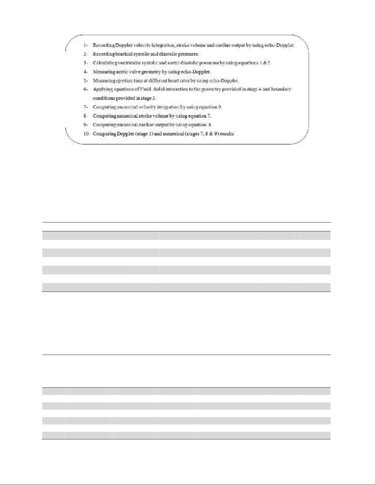
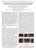
Workflow of the study was briefly provided in Fig. 1. Seven healthy subjects, aged 33 to 56 years
old, participated in this study with their hemodynamic data recorded during rest. Informed consent
was gained for the participants according to protocols confirmed by the Department of
Cardiovascular Imaging (Atherosclerosis research centre, Tehran, Iran). Following clinical
examination, the subjects were found to perform normal cardiovascular functions. Systolic and
diastolic pressures of the brachial artery were obtained (Table 1). Eq. (1) and Eq. (2) were applied to
measure the central pressure respecting to brachial pressure measurements (Park et al., 2011).
Central systolic pressure
≈
Brachial systolic pressure + 2.25, (1)
Central diastolic pressure
≈
Brachial diastolic pressure – 5.45, (2)
where all pressures were measured in mmHg.
A. Khosravi et al. / Engineering Solid Mechanics 2 (2014)
93
Fig. 1. workflow of study
As well as this, left ventricular systolic pressure was gained from the calculated central systolic
pressure. A pressure difference of around 5 mmHg was previously reported between peak left
ventricular systolic pressure and central systolic pressure, using catheterization (Laske et al., 1996).
The ejection times were also obtained from Doppler-flow imaging under B-mode.
Table 1
Systolic, diastolic pressures and ejection time for each subject
Subject HR ET LBSP LBDP VSP CDP
1
80 243 124 86 132 70
2
74 303 118 80 126 64
3 70 288 115 76 123 60
4 77 273 133 83 141 67
5
52 240 113 58 121 42
6
59 303 98 65 106 49
7 74 245 110 80 118 64
HR: Heart rate;
ET: Ejection time;
LBSP: Left brachial systolic pressure;
LBDP: Left brachial diastolic pressure;
VSP: Ventricular systolic pressure;
CDP: Central diastolic pressure;
Table 2
Geometric data of the aortic valves
Subject
Maximum
diameter of
normal aortic root
(mm)
Ventricular
side diameter
(mm)
Aortic side
diameter
(mm)
Ascending aorta diameter
after sinotubular junction
(mm)
Leaflet’s
length
(mm)
Valve’s
height
(mm)
1
29.7
20.5
25.1
31.6
12.6
21
2 33.8 23.1 30.3 35.4 14.9 27.4
3 33.9 21 30 35.9 14.5 30.9
4 28 20 26.6 31.7 10.8 20.6
5
29.4
19.4
26.5
31.3
10.6
19.1
6
26.5
20
26.6
31.7
10.4
19.8
7 29 19.2 25.2 28.5 11.5 19.3
94
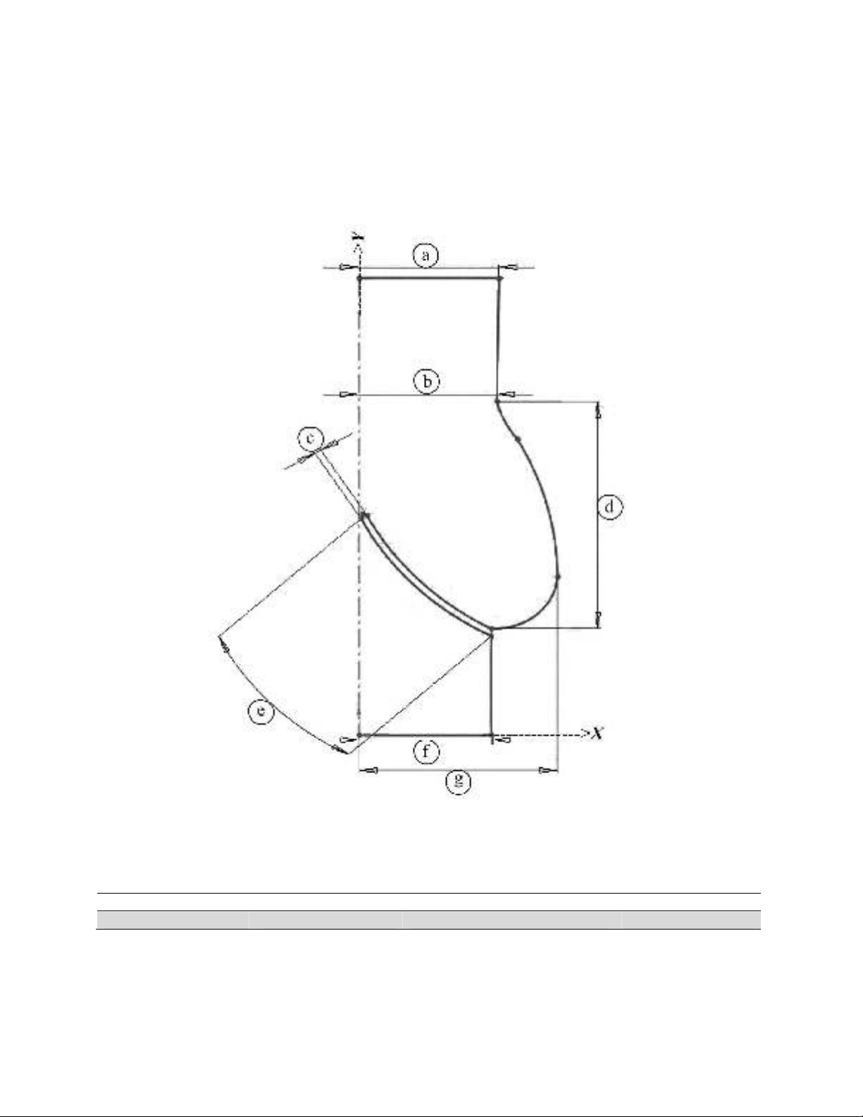
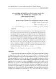
The aortic valve geometries modelled are presented in Fig. 2 and dimensions are provided in
Table 2. Dimensions were gained regarding T-wave and T-wave time of ECG. The two cusps were
taken into account to be homogenous, isotropic and to have a linear stress-strain relationship. This
assumption has been used in other heart valve models (De Hart et al., 2000; Espino et al., 2012 a,b;
Weinberg & Kaazempur-Mofrad, 2008). Blood was also supposed to be Newtonian and an
incompressible fluid (Pedley et al., 1978). All material properties are provided in Table 3 and were
obtained from the literature (Govindarajan et al., 2010; Koch et al., 2010).
Fig. 2. Aortic valve model
Table 3
Mechanical properties
Viscosity (Pa.s) Density (kg/m3) Young’s modulus (N/m2) Poisson ratio
3.5 x 10
-
3
1056 6.885 x 10
6
0.4999
For fluid boundaries (Fig. 2), pressure was used at the inflow boundary of the aortic root at the left
ventricular side. A moving ALE mesh was applied which enabled the deformation of the fluid mesh
to be tracked without the need for re-meshing (Weinberg & Kaazempur-Mofrad, 2008). Second order
A. Khosravi et al. / Engineering Solid Mechanics 2 (2014)
95
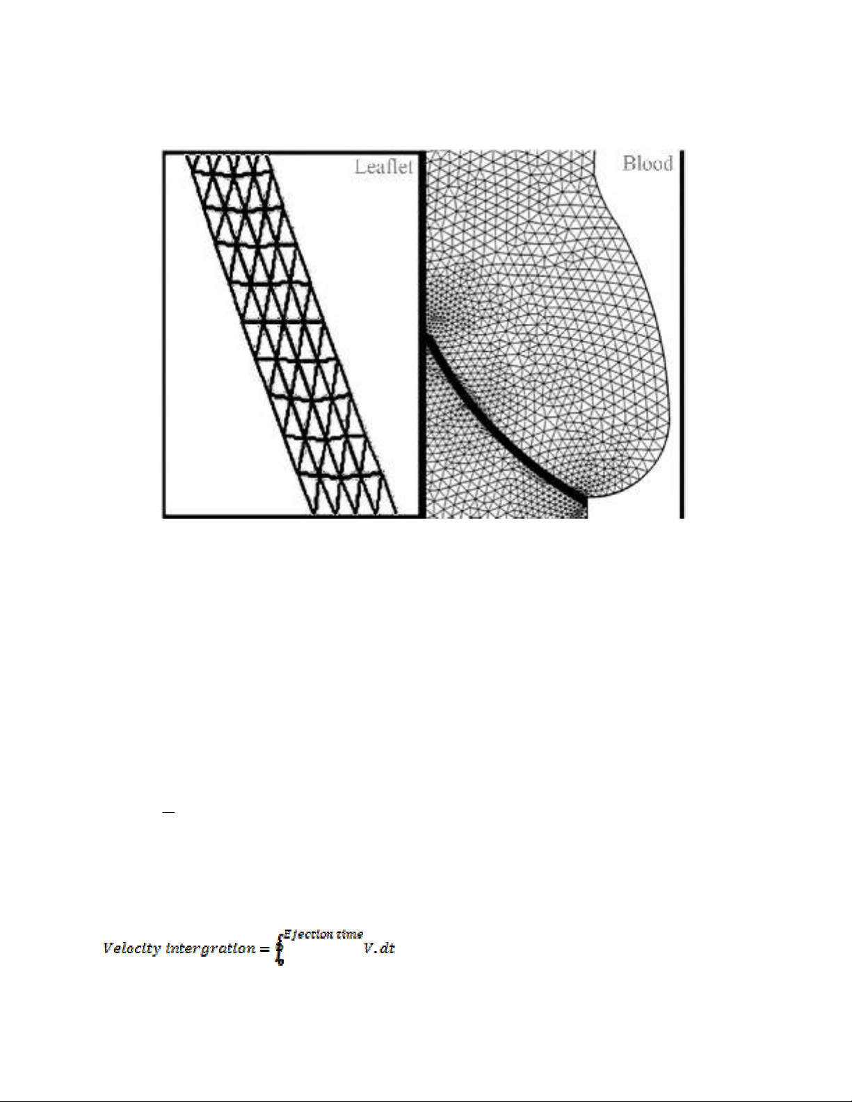
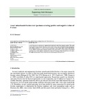
Lagrangian elements were used to define the mesh (Fig. 3). The finite element analysis package
Comsol Multi-physics (v4.2, Comsol Ltd, Cambridgeshire, UK) was used to solve the FSI model
under time dependent conditions (Espino et al., 2012a; Formaggia & Nobile, 1999).
Fig. 3. Mesh model
2.3. Analysis of fluid dynamics
Cardiac output was calculated applying Eq. (3):
Cardiac output = Stroke volume × Heart rate, (3)
where the stroke volume was computed from ECG using Eq. (4):
Stroke volume = Velocity integration × Aortic area, (4)
where the velocity integration was automatically acquired by tracing the Doppler flow from
ultrasound imaging. The aortic area was calculated utilizing Eq. (5):
2
2
D
Area
, (5)
where D is the calculated ascending aortic diameter after the sinotubular junction (Table 2). For FSI
simulations, the mean velocity numerically was obtained at each time step of the ejection period. Eq.
(6), however, was used to determine the velocity integration (used to determine both stroke volume
and cardiac output).
(6)


![Giáo trình Cấu trúc dữ liệu và giải thuật - Trường CĐ Cơ điện Hà Nội [Mới nhất]](https://cdn.tailieu.vn/images/document/thumbnail/2026/20260323/lionelmessi01/135x160/58171774381670.jpg)


![Giáo trình Tiện nâng cao (Nghề Cắt gọt kim loại, Trình độ Cao đẳng) - Trường Cao đẳng Cơ điện Hà Nội [Mới nhất]](https://cdn.tailieu.vn/images/document/thumbnail/2026/20260323/lionelmessi01/135x160/48101774403543.jpg)


