* Corresponding author
E-mail address:hrp07@ganpatuniversity.ac.in (H. Patel)
© 2019 by the authors; licensee Growing Science, Canada
doi: 10.5267/j.uscm.2018.4.002
Uncertain Supply Chain Management 7 (2019) 97–108
Contents lists available at GrowingScience
Uncertain Supply Chain Management
homepage: www.GrowingScience.com/uscm
Pricing model for instantaneous deteriorating items with partial backlogging and different demand
rates
Hetal Patel*
U. V. Patel College of Engineering, Ganpat University, India
C H R O N I C L E A B S T R A C T
Article history:
Received December18, 2017
Accepted April 20 2018
Available online
April 20 2018
In this study, a single product is considered which starts to deteriorate with constant rate of
replenishment and demand rate is time and price dependent exponential function. Shortage is
allowed with partial back logging and the relationship between backorder rate and waiting time
is considered to be exponential. The aim is to decide pricing strategy and maximize total
average profit function. Total profit function is optimized analytically and proved to be
concave function of price. Finally, numerical example is given to illustrate the implementation
of the algorithm followed by the sensitivity analysis.
ensee Growin
g
Science, Canada
by
the authors; lic9© 201
Keywords:
Instantaneous deterioration
Price discount
Back order, profit
Price and time dependent
1. Introduction
Product deterioration is very critical issue in various systems using inventory (Bakker et al., 2012).
Deterioration is considered as damage, vaporization, dryness, spoilage, etc. Blood bank, volatile
liquids, medicine, food stuff are deteriorating inventory goods, which deteriorate during their storage
period (Dye et al. 2007; Goyal & Giri, 2001). Loss due to deterioration cannot be negligible. Ghare and
Schrader (1963) initiated the journey of studying deteriorating inventory product by developing a
model for deteriorating inventory item with no shortage and constant deterioration rate. However,
against the assumption of constant deterioration rate, Covert and Philip (1973) relaxed this assumption
and developed a model by considering two-parameter Weibull distribution deterioration rate (Ouyang
et al., 2006). The literature is further extended by Philip (1974) by taking two-parameter Weibull
deterioration rate. Further, Aliyu and Boukas (1998) presented discrete-time inventory control problem
with deterministic or stochastic demand for deteriorating items having variable deterioration rate.
However, Chang and Dye (2001) described EOQ model taking varying deterioration rate of time and
allowing permissible delay in payments. Apart, Maity and Maiti (2009) explained multi-item inventory
model with real time examples having substitute and complimentary deteriorating items.

98
Distinctively, Mishra and Shah (2008) modeled salvage value taking demand constant and two variable
Weibull distribution function of time for varying deterioration rate, having no shortage. Ouyang et al.
(2009) formulated EOQ policy assuming demand rate as constant and non-instantaneous deterioration
rate as constant with no shortages. Allowing shortages reduces carrying costs and increases the cycle
time. If shortage cost is less than carrying cost then lowering the average inventory level by permitting
shortage, makes sense. This model allows shortages with partial backlogging. Li et al. (2007)
formulated model by considering demand rate as constant and also the deterioration rate as constant
having shortage with complete backlogging with postponement strategy. Taleizadeh and Nematollahi
(2014) developed a model by allowing delay in payment, complete back logging with constant
deterioration rate, and demand rate.
As constant demand is not possible in real and pricing decision is very critical for maximizing the
profit, many researchers have adopted pricing strategy with different assumption and conditions. In this
context, Abad (2001) developed an inventory model by taking demand as general function of price with
time dependent deterioration and shortages are partially backordered. The backlogging rate sometimes
behaves exponentially. Abad (2003) developed integrated pricing model allowing backlogging without
calculating backorder cost and the lost sale cost. Teng et al. (2007) extended Abad’s (2003) model by
calculating backlogging cost and lost sale cost in profit function. Shah et al. (2012) formulated
integrated ordering and pricing policy with quadratic demand function of time and power function of
price without allowing shortages and deterioration. Mukhopadhyay et al. (2004) computed demand rate
as general function of price and deterioration rate as time dependent linear function without provision
of shortages. Maihami and Abadi (2012) formulated pricing model by assuming demand as linear
function of price and power function of time allowing partial backlogging for non-instantaneous
deteriorating product.
Chang et al. (2006) gave pricing policy with constant deterioration rate for finite planning horizon
allowing partially backlogging. Widyadanaa et al. (2011) considered finite planning horizon for
instantaneous deterioration with planned backlogging. Furthermore, Chang et al. (2006) further
examined the EOQ model by taking backorder rate in general form and importantly taken demand as
stock dependent. The condition of partial backlogging was relaxed in a study by Dye et al. (2007) to
develop pricing strategy by considering full backlogging. In fact, seasonality aspect was considered
while developing EOQ model in a multi-echelon system with constant deterioration and partial
backlogging. Still, studies performed have overlooked the situations when demand is stock dependent.
Guchhait et al. (2013) formulated Lot sizing model with constant deterioration.
Distinctively, Panda et al. (2009) approached a model using selling price discounts along with demand
as stock dependent. Wang and Huang (2014) constructed pricing model considering ramp-type
dependent demand. Inventory dependent demand with constant rate of deterioration was considered in
Tripathi and Mishra (2014) study. Farughi et al. (2014) modeled the inventory system for non-
instantaneous deteriorating items where demand is linear function of price and exponential function of
time with constant deterioration rate. They also allowed shortages partially with back order rate in
fraction form. Kumar and Kumar (2016) studied the salvage worth and learning by considering partial
shortages, Tripathi and Kaur (2017) considered time-shortages, which is non-increasing and
interestingly since they assumed deterioration as time dependent, which is non-decreasing. Apart, Saha
and Sen (2017) studied deterioration as probabilistic with backlogging and demand as negative
exponential. Differently, Shah (2017) formulated model taking fixed lifetime with conditional trade
credit, however Pandey et al. (2017) offered quantity discounts while, Rastogi et al. (2017) offered
credit limits with case discount. Recently, Mashud et al. (2018) used products with different
deterioration rates allowing shortages and demand as stock and price dependent.

H. Patel / Uncertain Supply Chain Management 7 (2019)
99
Among all above literature, very few studies are offering pricing discount. In current study demand rate
is different in various time interval where demand depends on price and time exponentially and
discounts offering on price during shortages. Shortages are partially backlogged where back order rate
is exponential function of waiting time. We consider price discounts and study the effect of weighting
coefficient of price on total profit. Notations and assumptions are outlined in the next section. Then,
total profit function is optimized theoretically and proved to be a concave function of price and time.
Finally, procedure for solving a model is demonstrated through numerical analysis to illustrate
algorithm and sensitivity analysis is presented.
2. Notations and assumptions
The assumptions with some notations are listed as follow:
2.1 Notations
p
selling price / unit (decision variable)
w weighting coefficient
01w
,
D
pt demand function at time t for given
p
p
c purchasing cost /unit
0p
cp
1
t point of time where inventory is zero (decision variable)
2
t time duration of shortages (decision variable)
h cost of holding / unit /unit time
K
cost of ordering / order
s
c backorder cost / unit /unit time
o cost of lost sales / unit
M
I Level of maximum inventory at each cycle
Q ordering quantity / cycle
S
maximum shortage
1
I
t inventory at time
1
0ttt where deterioration exists
2
I
t inventory at time
2
0ttt is negative
2.2 Assumptions
1. Single item instantaneous deterioration with constant rate
, is considered.
2. Infinite replenishment rate is considered with finite order size.
3.
,
D
pt is a “demand function of selling price and time”, and is computed by
1
12
, if 0
,, if 0
dpft t t
Dpt dp t t
where 1
() , () , (0 1)
bt
dp ap ft e p pw w
4. There is no provision for replacing or repairing of deteriorated units.
5. Backlogging rate is
x
x
e
as shortages are allowed, where
x
is the waiting time up to the next
arrival.

100
3. Model Formulation
Let
M
I
units of items arrive at the inventory system at the beginning of replenishment cycle. The
inventory level declines during time 0 to 1
t, only due to demand rate and deterioration rate to be zero
and shortages start during time 0 to 2
twhich are backlogged partially. The process is repeated as
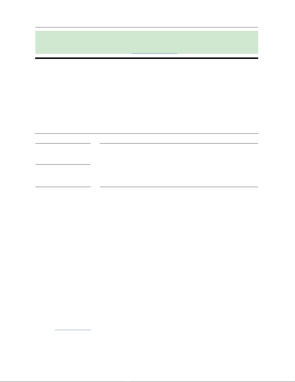
mentioned above. The model is followed as per following Fig. 1.
Fig. 1. The inventory system
As the nature of deteriorating inventory item, inventory model is characterized by following differential
equation:
1
11
, 0
bt
dI t It ape t t
dt
(1)
2
2
2
e, 0
btt
dI t apw t t
dt
(2)
With terminal condition,
10
M
I
I and
11 21
0
I
tIt (3)
By solving equations (1) and (2), we get
11
, 0
bt t
M
ap e e
I
tI tt
(4)
2
22
ee1, 0
b
tt
apw
It tt
(5)
Since
11 21 0It It
, it follows from Eq. (3) and Eq. (4) that, (6)
0
Inventory Level
On-hand
Inventory
Ordering
Quantity
Lost sales
Backorders
2
t
T
1
t

H. Patel / Uncertain Supply Chain Management 7 (2019)
101
Here, maximum inventory level is
11
tt
b
M
ap e e
I
. Put this value in Eq. (3), we get
11
1 1
, 0
tt
bbt t
ap e e ap e e
I
ttt
(7)
The maximum shortages is
2
22 1e
b
t
apw
SIt
(8)
Thus, the order quantity per order is
11
2
1e
tt b
b
t
M
ap e e apw
QI S
(9)
To compose profit function, following elements are needed:
The ordering cost is OC K
The purchase cost is
11
2
1
tt b
b
t
pp
ap e e apw
PC c Q c e
The holding cost is
1
1
1
11 1 1
1
0
1
t
t
b
t
tt t t
HC h I t dt
hap e te e e e e
Considering backlog, the cost of shortage is
22
22
22
0
1
btt
ts
s
ca pw e e t
SC c I t dt
Realizing lost sales, the opportunity cost is computed as
2
2
12
0
2
1
1
t
b
t
LC od p t t dt
oa pw et
The sales revenue is
1
12
0,
11
t
tt
b
b
SR p D p t dt S
ee
pap apw
Gathering above element, the total average profit (denoted by
12
,,
Apt t) is computed as,
12
12
12
,,
,,
A
pt t
pt t tt
, (10)