http://www.iaeme.com/IJMET/index.asp 603 editor@iaeme.com
International Journal of Mechanical Engineering and Technology (IJMET)
Volume 10, Issue 3, March 2019, pp. 603–613, Article ID: IJMET_10_03_062
Available online at http://www.iaeme.com/ijmet/issues.asp?JType=IJMET&VType=10&IType=3
ISSN Print: 0976-6340 and ISSN Online: 0976-6359
© IAEME Publication Scopus Indexed
PROFIT AGENT CLASSIFICATION USING
FEATURE SELECTION EIGENVECTOR
CENTRALITY
Zidni Nurrobi Agam
Computer Science Department, Bina Nusantara University,
Jakarta, Indonesia 11480
Sani M. Isa
Computer Science Department, Bina Nusantara University,
Jakarta, Indonesia 11480
Abstract
Classification is a method that process related categories used to group data
according to it are similarities. High dimensional data used in the classification
process sometimes makes a classification process not optimize because there are huge
amounts of otherwise meaningless data. in this paper, we try to classify profit agent
from PT.XYZ and find the best feature that has a major impact to profit agent. Feature
selection is one of the methods that can optimize the dataset for the classification
process. in this paper we applied a feature selection based on graph method, graph
method identifies the most important nodes that are interrelated with neighbors nodes.
Eigenvector centrality is a method that estimates the importance of features to its
neighbors, using Eigenvector centrality will ranking central nodes as candidate
features that used for classification method and find the best feature for classifying
Data Agent. Support Vector Machines (SVM) is a method that will be used whether
the approach using Feature Selection with Eigenvalue Centrality will further optimize
the accuracy of the classification.
Keywords: Classification, Support Vector Machines, Feature Selection, Eigenvalue
Centrality, Graph-based.
Cite this Article: Zidni Nurrobi Agam and Sani M. Isa, Profit Agent Classification
Using Feature Selection Eigenvector Centrality, International Journal of Mechanical
Engineering and Technology (IJMET)10(3), 2019, pp. 603–613.
http://www.iaeme.com/ijmet/issues.asp?JType=IJMET&VType=10&IType=3

Zidni Nurrobi Agam and Sani M. Isa
http://www.iaeme.com/IJMET/index.asp 604 editor@iaeme.com
1. INTRODUCTION
In this era data is a very important commodity used in almost all existing technologies, data
makes researchers examine more data in order to find hidden patterns that can be used as
information. but with the increasing number of data, there are also many data that irrelevant
and redundant dataset, making the quality of the data less good.
Feature Selection is a method that selects a subset of variables from the input which can
efficiently describe the input data while reducing effects from noise or irrelevant variables and
still provide good prediction results [1]. Usually, feature selection operation both ranking and
subset selection [2][3] to get most relational or most important value from a dataset. n
described as total feature the goal of feature selection is to select the optimal feature I, so the
optimal feature selection is I < n. With Feature Selection processing data will improve the
overall prediction because optimal dataset that improves by feature selection.
we applied feature selection for optimizing classification based on graph feature selection,
this feature selection ranked feature based on Eigenvector Centrality. in graph theory, ECFS
measures a node that has major impact on other nodes in the network. all nodes on the
network are assigned relative scores based on the concept that nodes that have high value
contribute more to the score of the node in question than equal connections to low-scoring
nodes [4]. A high eigenvector score means that a node is connected to many nodes who
themselves have high scores. so, relationship between feature (nodes) are measure by weight
the connection between nodes. The problem from feature subset selection refers the task of
identifying and selecting a useful subset of attributes to be used to represent patterns from a
larger set of often mutually redundant, possibly irrelevant, attributes with different associated
measurement costs and/or risks [5]. we try to find the most influential feature to predict the
profit agent with ECFS.
There are many studies that research about Eigenvector Centrality such as Nicholas J.
Bryan and Ge Wang [6] , Nicholas J. Bryan and team research about how music with so
many features can create pattern network between song and used to help describe patterns of
musical influence in sample-based music suitable for musicological analysis. [7] To analyze
rank influence feature between genre music with Eigenvector Centrality. and on 2016
Giorgio Roffo & Simione Melzi research about Feature ranking vie Eigenvector Centrality, in
Giorgio Roffo & Simione Melzi research important feature by identifying the most important
attribute into an arbitrary set of cues then mapping the problem to find where feature are the
nodes by assessing the importance of nodes through some indicator of centrality. for building
the graph and the weighted distance between nodes Giorgio Roffo & Simione Melzi use
Fisher Criteria.
The Goal of this paper is to applied Chi-Square and ECFS feature selection and compare
both features with different dataset. Both Feature Selection test with HCC and Profit agent
dataset, this test validates with K Fold Cross Validation feature selection to test the model’s
ability then evaluated with confusion matrix to measure misclassification. Based on ECFS
results we try to determine which attribute from profit agent that have a major impact on
another attribute on profit agent dataset.
2. RESEARCH METHOD
A discussion about Feature selection and ranking based on Graph network [8] method will be
discussed in this paragraph. To build the graph first we have to define how to design and build
the graph.

Profit Agent Classification Using Feature Selection Eigenvector Centrality
http://www.iaeme.com/IJMET/index.asp 605 editor@iaeme.com
2.1. Graph Design
Define the graph G = (V,E), V is a vertices corresponding one by one to each variable x, x is a
set of features X = {x(1),x(2),.....x(n)}. E define as a (Weight) edges between nodes (features).
To represent the graph that have relationship between edge. Define node (feature) into
adjency matrix represent on binary matrix:
αij = ℓ(x(i),x(j)) (1)
When the graph not complex, the adjacency matrix are 0 all 1 or (there are no weights on
the edges or multiple edges) and the diagonal entries are all [9] , but if the adjacency matrix
has weighted on edges the adjacency matrix will not 0 and 1 but fill with weighted as figure 1.
(
)
(
)
Figure 1 Matrix A with Weight and Matrix A no Weight
A design graph is a part to weight the graph according to how good the relationship
between two feature in the dataset. we apply Fisher linear discriminant [10] to find the mean
and standard deviation, this methods find a linear combination of features which characterizes
or separates two or more classes of objects or events.
( ) | |
(2)
Where:
m = represent a mean.
s = represent a variance. (standard deviation)
Subscripts = the subscripts denote the two classes.
After we measure the relationship between to class and we get the weight from fisher
linear Discriminant, then we implement Eigenvector Centrality to rank and filter data from
spearman correlation weight that generated from the relationship between 2 nodes (feature).
For G: = (V, E) with |V| vertices let A = (av,t) adjacency matrix, the relative centrality score of
vertex v can be defined as :
∑
( )
∑ (3)
where M(v) is a set of the neighbors of and is a constant. With a small rearrangement
this can be rewritten in vector notation as the eigenvector equation:
(4)
However, as we count longer and longer paths, this measure of accessibility converges to
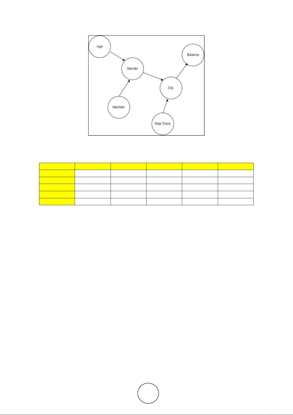
an index known as eigenvector centrality measure (EC). Example for node and adjacency
matrix [9] described in figure 2 and Table 1.
Zidni Nurrobi Agam and Sani M. Isa
http://www.iaeme.com/IJMET/index.asp 606 editor@iaeme.com
Figure 2 Node Data Agent Company XYZ
Table 1 Example adjacency Matrix
Example
Age
Gender
City
Balance
Total Trans
Age
0
8.56
0
0
0
Gender
0
0
3.4
7.4
0
City
0
8.56
0
2.6
0
Balance
0
7.4
2.6
0
0
Total Trans
0
0
8.7
0
0
2.2. SVM Classification Method
SVM Classification is classification analysis which fall into the category a supervised
learning algorithm. Given a set of training examples, each marked as belonging to one or the
other of two categories, Support vectro machine builds a model that assigns new examples to
one category or the other, making it a non-probabilistic binary linear classifier. Its basic idea
is to map data into a high dimensional space and find a separating hyperplane with the
maximal margin. Given a training dataset of n points of the form:
( ) (
) (5)
where the are 1 or −1 [11], each point indicating the class to which the point
belongs. Each
is p-dimensional real vector. We want to find the "maximum-margin
hyperplane" that divides the group of points
for which = 1 from the group of points for
which = - 1 which is defined so that the distance between the hyperplane and the nearest
point from either group is maximized.
Profit Agent Classification Using Feature Selection Eigenvector Centrality
http://www.iaeme.com/IJMET/index.asp 607 editor@iaeme.com
Figure 3 SVM try to find best Hayperlane to split class -1 and + 1
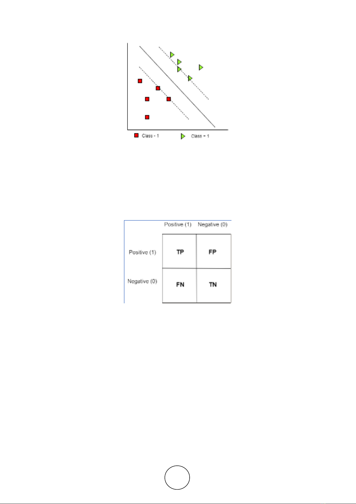
2.3. Confusion Matrix
To measure how to optimize SVM Classification used Eigenvector Centrality, we used a
confusion matrix, confusion matrix is a table that is often used to describe the performance of
a classification model (or "classifier") on a set of test data for which the true values are
known. The table of confusion matrix will describe on figure 4 there is a TP (True Positives),
TN (True Negatives), FP (False Positives) and FN (False Negatives).
Figure 4 Confusion Matrix
True Positive: We predicted yes (they have failure), and they do have the failure.
False Positives: We predicted yes, but they don't actually have the failure.
True Negatives: We predicted no, and they don't have the failure.
False Negatives: We predicted no, but they actually do have the failure.
3. RESULT & ANALYSIS
In this step we discuss result from compare between Eigenvector Centrality FS and Chi-
Square FS, then we used Support Vector Machines Classification to calculate and compare
accuracy between that feature selection.
3.1. Dataset
Dataset PT. XYZ is chosen analysis feature selection Eigenvector Centrality with the
scenario. first, we describe the dataset used for feature selection as how many features used
for prediction, data agent is a categorical data collected from transaction data and have 6
attributes that used for analysis: