Statistical Concepts in Metrology_1

Chia sẻ: Thao Thao | Ngày: | Loại File: PDF | Số trang:12

Thêm vào BST

Báo xấu

42
lượt xem 2
download

Download Vui lòng tải xuống để xem tài liệu đầy đủ

Trong các mảng không có hai khả năng có chính xác cùng một giá trị. Từ Định lý giới hạn trung tâm, nó có thể được suy luận rằng sẽ được khoảng bình thường được phân phối với aj.. / fl.: Độ lệch chuẩn.

Chủ đề:

Bình luận(0) Đăng nhập để gửi bình luận!

Lưu

Nội dung Text: Statistical Concepts in Metrology_1

~. ~(-", ~ ' " """"'- '" Simpo PDF Merge and Split Unregistered Version - http://www.simpopdf.com NBS Special 747 Publication Statistical With a Postscript Concepts in Metrology on Statistical Graphics Harry H. Ku Statistical Engineering Division Center for Computing and Applied Mathematics National Engineering Laboratory National Bureau of Standards Gaithersburg, MD 20899 August 1988 "'~' OF ;t "'\\1/ ~ :l 1!J~ii' L eo...u Of ~ S. Department of Commerce C. William Verity, Secretary National Bureau of Standards Ernest Ambler Director
Simpo PDF Merge and Split Unregistered Version - http://www.simpopdf.com For sale by the Superintendent u.S. Government Printing Office Library of Congress of Documents Catalog Card Number: 88-600569 Washington: 1988 u.S. Government Printing Office National Bureau of Standards Washington, DC .20402 Special Publication 747 Nati. Bur. Stand. (U. Spec. Pubi. 747, 48 pages (Aug. 1988) COD EN: XNBSAV
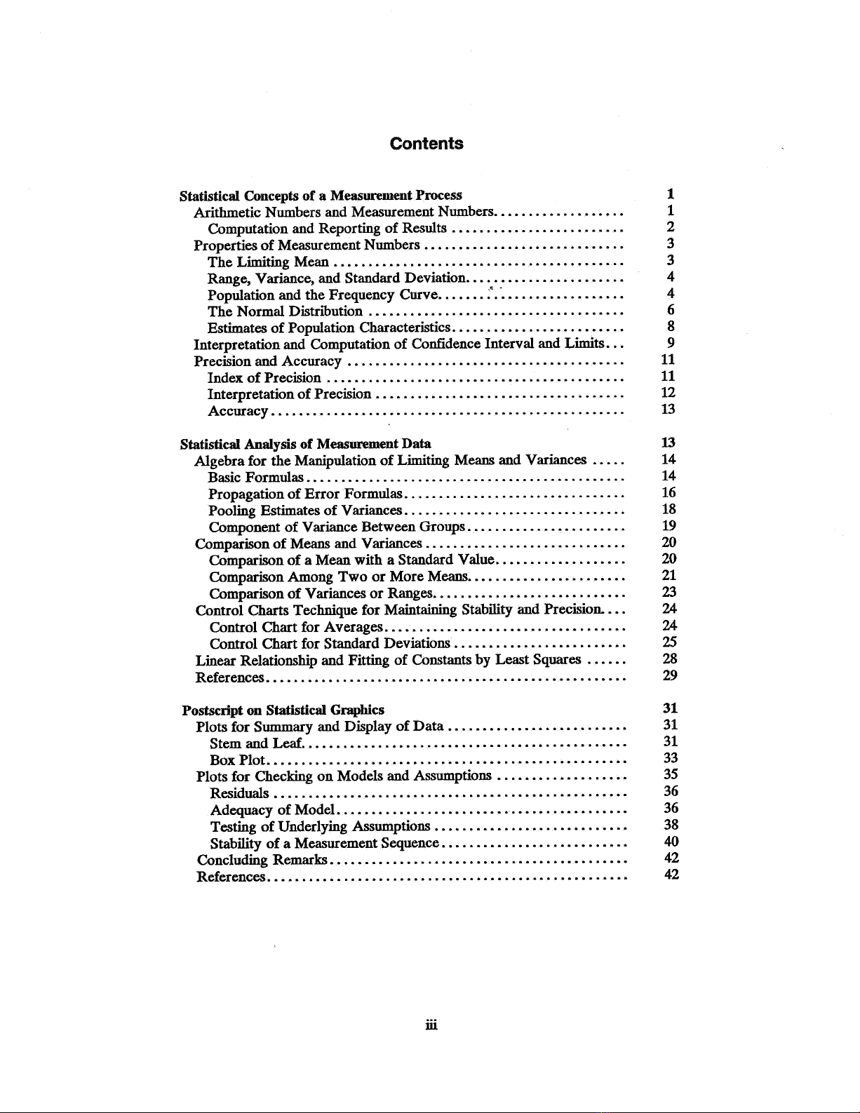
..................................... ............................................ ........................................... .... ..............................: ..... ........ .......... ..... .... . . . . . . . . . . . . . '. . . . . Simpo PDF Merge and Split Unregistered Version - http://www.simpopdf.com Contents Statistical Concepts of a Measurement Process Arithmetic Numbers and Measurement Numbers. . . . . Computation and Reporting of Results. . . . Properties of Measurement Numbers. . . . . The Limiting Mean Range, Variance, and Standard Deviation. . . . . Population and the Frequency Curve. . . . The Normal Distribution Estimates of Population Characteristics. . . . . Interpretation and Computation of Confidence Interval and Limits. . . Precision and Accuracy " Index of Precision Interpretation of Precision. . . . Accuracy. Statistical Analysis of Measurement Data Algebra for the Manipulation of Limiting Means and Variances. . . . . BasicFormulas.............................................. Propagation of Error Formulas. ... .. . .. . . .. Pooling Estimates of Variances. . . . Component of Variance Between Groups..................... Comparison of Means and Variances... Comparison of a Mean with a Standard Value. Comparison Among Two or More Means. . Comparison of Variances or Ranges. . . . . Control Charts Technique for Maintaining Stability and Precision. . . Control Chart for Averages. .. . . . Control Chart for Standard Deviations. . . . Linear Relationship and Fitting of Constants by Least Squares. . . . . References........... Postscript on Statistical Graphics Plots for Summary and Display of Data. . . Stem and Leaf............ ............. BoxPlot......... ...... Plots for Checking on Models and Assumptions. . . . Residuals " Adequacy of Model. Testing of Underlying Assumptions. . . . . Stability of a Measurement Sequence. . . . . Concluding Remarks.. References... ........ ........,... ... ill
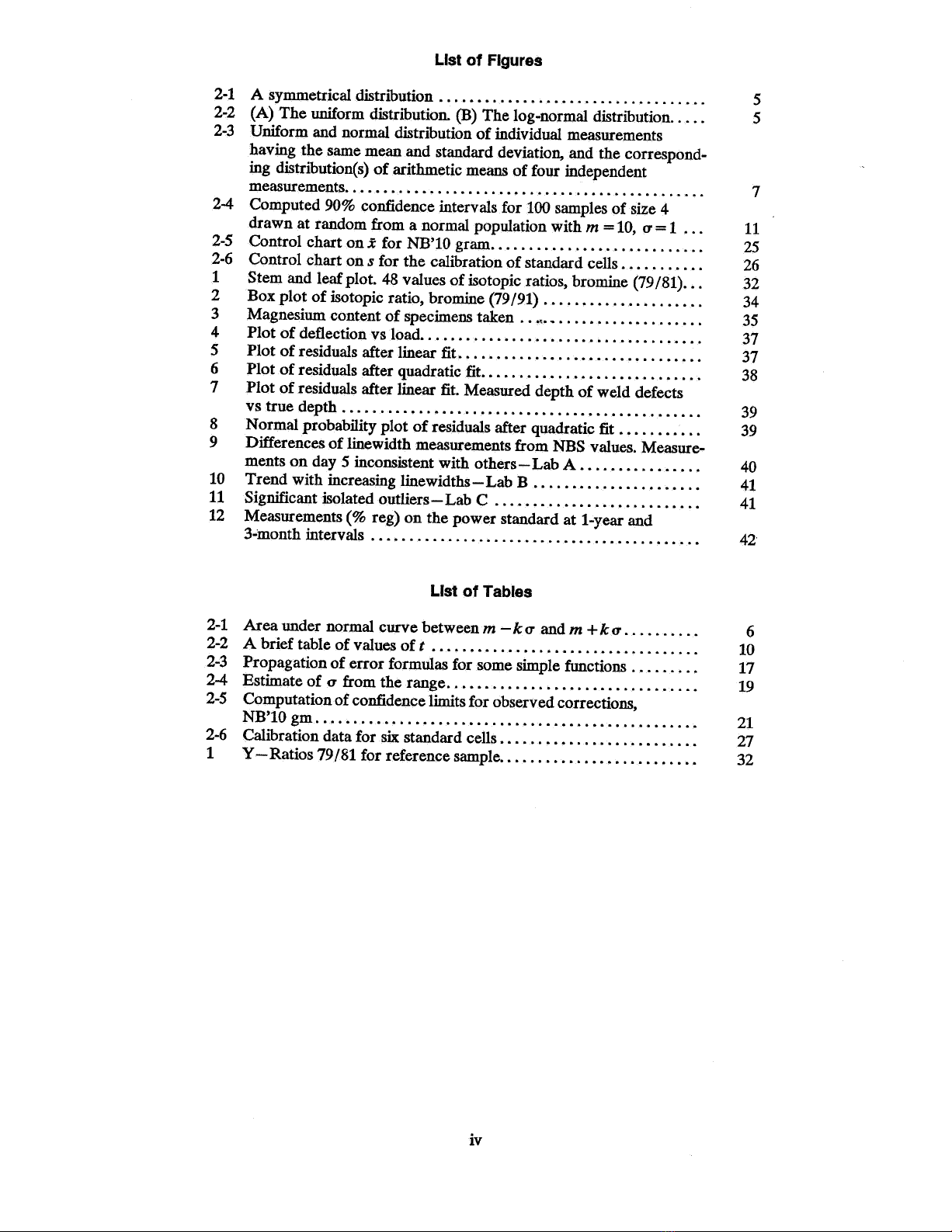
............................................. . .... .". ............,.............. .. .........,....... .. ..............................'............................... .. ......,..... .... .. '." .... . .. LIst of Figures Simpo PDF Merge and Split Unregistered Version - http://www.simpopdf.com 1 A sYIllDletrical distribution " (A) The uniform. distribution. (B) The log-normal distribution. . . . . Uniform and normal distribution of individual measurements having the same mean and standard deviation, and the correspond- ing distribution(s) of arithmetic m.eans of four independent measurements................................................. 2-4 Computed 90% confidence intervals for 100 samples of size 4 = 10, 0' = 1 '" drawn at random from a normal population with Control chart on.f for NB' 1O gram. . Control chart on 8 for the calibration of standard cells. . . . . Stem and leaf plot. 48 values of isotopic ratios, bromine (79/81). Box plot of isotopic ratio, bromine (79/91) Magnesium content of specimens taken. . ... Plotofdeflectionvsload.................................."'" Plot ofresiduals after linear fit. .. . . Plot ofresiduals after quadratic fit. . . . Plot of residuals after linear fit. Measured depth of weld defects vstruedepth................................................ Normal probability plot of residuals after quadratic fit Djfferences of linewidth measurements from NBS values. Measure- ments on day 5 inconsistent with others~ Lab A . . .. . . Trend with increasing linewidths - Lab B . . Significant isolated outliers- Lab C" Measurements (% reg) on the power standard at i-year and 3.;monthintervals LIst of Tables 1 Area m - kO' under normal curve between m +kO'.......... and 2 A brief table of values oft ................................... Propagation of error formulas for some simple functions. . . . . 2-4 Estimate of 0' from the range. . .. . .... . . . . Computation of confidence limits for observed corrections, 10gm.................................................... NB' Calibration data for six standard cells. . . 1Y~ for reference sample.. . '" Ratios 79181
Simpo PDF Merge and Split Unregistered Version - http://www.simpopdf.com Statistical Concepts in Metrology- With a Postscript on Statistical Graphics Harry H. Ku Statistical Engineering Division, National Bureau of Standards, Gaithersburg, MD 20899 Statistical Concepts in Metrology " was originally written as Chapter 2 for the Handbook of Industrial Metrology published by the American Society of Tool and Manufacturing Engineers, 1967. It was reprinted as one of 40 papers in NBS Special Publication 300, VolUlUe I, Precision Measurement and Calibration; Statistical Concepts and Procedures, 1969. Since then this chapter has been used as basic text in statistics in Bureau-sponsored courses and semi- nars, including those for Electricity, Electronics, and Analytical Chemistry. While concepts and techniques introduced in the original chapter remain valid and appropriate, some additions on recent development of graphical methods for the treatment . of data would be useful. Graphical methods can be used effectively to "explore" information in data sets prior to the application of classical statistical procedures. For this reason additional sections on statisti- cal graphics are added as a postscript. Key words: graphics; measurement; metrology; plots; statistics; uncertainty. STATISTICAL CONCEPTS OF A MEASUREMENT PROCESS and Measurement Arithmetic Numb~rs Numbers numbers are used for different purposes In metrological work , digital and consequently these numbers have different interpretations. It is therefore important to differentiate the two types of numbers which will be encountered. Arithmetic numbers are exact numbers. 3 J2, i, 7J: are all exact or r.umbers by definition , although in expressing some of these numbers in digital form , approximation may have to be used. Thus 7J: may be written as 3, 14 or 3. 1416, depending on our judgment of which is the proper one to use from the combined point of view of accuracy and convenience. By the
.. Simpo PDF Merge and Splitrounding, the approximations do not differ from the exact usual rules of Unregistered Version - http://www.simpopdf.com values by more than *0. 5 units of the last recorded digit. The accuracy of the result can always be extended if necessary. Measurement numbers , on the other hand , are not approximations to exact numbers , but numbers obtained by operation under approximately the same conditions. For example , three measurements on the diameter of a steel shaft with a micrometer may yield the following results: General notation No. in Diameter 396 392 401 Sum 1.189 i=1 ~~Xi Average 0.3963 = Xmax Range 0. 009 min There is no rounding off here. The last digit in the measured value depends on the instrument used and our ability to read it. If we had used a coarser instrument , we might have obtained 0.4 0.4 , and 0.4; if a finer instrument , we might have been able to record to the fifth digit after the decimal point. In all cases , however , the last digit given certainly does by less than not imply that the measured value differs from the diameter ::1:::0. 5 unit of the last digit. Thus we see that measurement numbers differ by their very nature from arithmetic numbers. In fact , the phrase .. significant figures " has little meaning in the manipulation of numbers resulting from measurements. Reflection on the simple example above will help to convince one of this fact. Computation and Reporting of Results. By experience , the metrologist can usually select an instrument to give him results adequate for his needs as illustrated in the example above. Unfortunately, in the process of com- putation , both arithmetic numbers and measurement numbers are present and frequently confusion reigns over the number of digits to be kept in successive arithmetic operations. No general rule can be given for all types of arithmetic operations. If the severe rounding would result in loss of infor- instrument is well-chosen , mation. One suggestion , therefore , is to treat all measurement numbers as exact numbers in the operations and to round off the final result only. Another recommended procedure is to carry two or three extra figures throughout the computation , and then to round off the final reported value to an appropriate number of digits. number of digits to be retained in the final result The .. appropriate " uncertainties " attached to this reported value. The term depends on the .. uncertainty " will he treated later under .. Precision .and Accuracy ; our only concern here is the number of digits in the expression for uncertainty. A recommended rule is that the uncertainty should be stated to no more than two significant figures, and the reported value itself should be stated
to the last place affected by the qualification given by the uncertainty state- Simpo PDF Merge andexample is: ment. An Split Unregistered Version - http://www.simpopdf.com The apparent mass correction for the nominal 109 weight is +0. 0420 mg with an overall uncertainty of ::1:0. 0087 mg using three effect of random errors of standard deviations as a limit to the measurement , the magnitude of systematic errors from known sources being negligible. The sentence form is preferred since then the burden is on the reporter to specify exactly the meaning of the term uncertainty, and to spell out its is the reported where h, 1: components. Abbreviated forms such as a measure of uncertainty in some vague sense , should always value and be avoided. Properties of Mecsurement Numbers The study of the properties of measurement numbers , or the Theory of Errors , formally began with Thomas Simpson more than two hundred years ago , and attained its full development in the hands of Laplace and Gauss. In the next subsections some of the important properties of measurement numbers will be discussed and summarized , thus providing a basis for the statistical treatment ' and analysis of these numbers in the following major section. The Limiting Mean. As shown in the micrometer example above, the repeated measurements of a single physical quantity under essentially results of measurement numbers. Each member of yield a set of the same conditions this set is an estimate of the quantity being measured , and has equal claims measurements on its value. By convention , the numerical values of these and the range by x, Xn, X2'.' the arithmetic mean by are denoted by Xh largest value and the smallest value , the difference between the measurements. obtained in the If the results of measurements are to make any sense for the purpose at hand , we must require these numbers , though different , to behave . as a group in a certain predictable manner. Experience has shown that this indeed the case under the conditions stated in italics above. In fact , let us adopt as the postulate of measurement a statement due to N. Ernest Dorsey (reference 2): The mean ora family of measurements-of a number of measure- ments for a given quantity carried out by the same apparatus, pro- cedure , and observer-approaches a definite value as the number of measurements is indefinitely increased. Otherwise, they could not properly be called measurements of a given quantity. In the theory of errors , this limiting mean is frequently called the ' true ' value although it bears no necessary relation to the true quaesitum, to the actual value of the quantity that the observer desires to measure. This has often confused the unwary. Let us call it the limiting mean. postulate, there exists a limiting mean Thus, according to this approaches as the number of measurements increases indefinitely, which 00. Furthermore , if the true value is 7 , there as , in symbols - 7 , where A is defined and 7 , or A = is usually a difference between measurements. as the bias or systematic error of the *References ' are listed at the end of this chapter.
"::::: In practice , however , we will run into difficulties. The value of cannot Simpo PDF Merge and Split since one cannot make http://www.simpopdf.com be obtained Unregistered Version -an infinite number of measurements. Even for a large number of measurements , the conditions will not remain constant , since changes occur from hour to hour , and from day to day. is unknown and usually unknowable , hence also the bias. The value of Nevertheless , seemingly simple postulate does provide a sound foun- this dation to build on toward a mathematical model , from which estimates can be made and inference drawn , as will be seen later on. measurements flange, Variance, and Standard Deviation. The range of on the other hand , does not enjoy this desirable property of the arithmetic mean. With one more measurement , the range may increase but cannot decrease. Since only the largest and the smallest numbers enter into its calculation , obviously the additional information provided by the measure- lost. It will be desirable ' to look for another measure ments in between is of the dispersion (spread , or scattering) of our measurements which will utilize each measurement made with equal weight , and which will approach a definite number as the number of measurements is indefinitely increased. A number of such measures can be constructed; the most frequently used are the variance and the standard deviation. The choice of the variance dispersion is based upon its mathematical convenience as the measure of and maneuverability Variance is defined as the value approached by the average of the sum of squares of the deviations of individual measurements from the limiting mean as the number of measurements is indefinitely increased , or symbols: in 2- ~ ------ 00 ------ (T (Xi m)2 variance, as The positive square root of the variance , (T is called the standard deviation (of a single measurement); the standard deviation is of the same dimension- ality as the limiting mean. There are other measures of dispersion , such as average deviation and probable error. The relationships between these measures and the standard deviation can be found in reference I. Population and the frequency We shall call the limiting mean Curve. the location parameter and the standard deviation (T the scale parameter the population of measurement numbers generated by a particular measure- ment process. By population is meant the conceptually infinite number of and (T describe measurements that can be generated. The two numbers this population of measurements to a large extent , and specify it completely in one important special case. Our model of a measurement process consists then of a defined popu- lation of measurement numbers with a and a standard limiting mean deviation (T. The result of a single measurement can take randomly any X* of the values belonging to this population. The probability that a particular measurement yields a value of which is the less than or equal to is proportion of the population that is less than or equal to in symbols PfX proportion of population less than or equal to to represent the value that might be *Convention is followed in using the capital produced by employing the measurement process to obtain a measurement (i. , a random observed. variable), and the lower case to represent a particular value of
Simpo PDF Merge and Split Unregistered Version -probability that Similar statements can be made for the http://www.simpopdf.com will be greater as follows: PfX than or equal to between and or for or Pfx For . a measurement process that yields numbers on a continuous scale for the population can be represented by the distribution of values of a smooth curve, for example , curve C in Fig. 2- 1. C is called a frequency curve. The area between C and the abscissa bounded by any two values is the proportion of the population that takes values between (xI and will assume values between the two values , or the probability that can be represented by and x2. For example, the probability that the total area between the frequency curve the shaded area to the left of and the abscissa being one by definition. Note that the shape of C is not determined by and (J' alone. Any curve C' enclosing an area of unity with the abscissa defines the distribution of a particular population. Two examples , the uniform distribution and the log-normal distribution are given in Figs. 2-2A and 2-28. These and other distributions are useful in describing .certain populations. +0" 30" 20" +30" +20" Ag. 2- 1. A synunetrical distribution. t20" 20" -0" +0" 20" 40" 60" 50- Ag. 2-2. (A) The uniform distribution (B) The log-normal distribution.
Simpo PDF Merge and Split Unregistered Version - http://www.simpopdf.comprocess For .data generated by a measurement The Normal Distribution. the following properties are usually observed: I. The results spread roughly symmetrically about a central value. 2. Small deviations from this central value are more frequently found than large deviations. A measurement process having these two properties would generate a fre- quencycurve similar to that shown in Fig. 2- 1 which is symmetrical and The study of a particular theoretical represen- m. bunched together about frequency curve of this type leads to the celebrated bell-shaped tation of a normal curve (Gauss error curve. Measurements having such a normal distributed, or distributed in frequency curve are said to be normally accordance with the normal law of error. The normal curve .can be represented , t:xactly by the mathematical expreSSIOn 1/2((x-m)'/u (2- J2it 71828 is the base of the abscissa and where is the ordinate and natural logarithms. Some of the important features of the normal curve are: 1. It is symmetrical about 2. The area under the curve is one , as required. is used as unit on the abscissa , then the area under the curve cr 3. If tabulated can be computed from cr between constant multiples of values of the normal distribution. In particular , areas under the curve are given in and kcr kcr for some useful intervals between Table 2- 1. Thus about two- thirds of the area lies within one cr of 3 percent beyond and less than 0. 2cr of more than 95 percent within 3cr from Table 2- 1. k CT (T and Area under normal curve between 2.58 1.96 6745 1.00 Percent area under 99. 95.5 99. 95. 68.3 50. curve (approx. 4. From Eq. (2-0), it is evident that the frequency curve is completely cr. and determined by the two parameters The normal distribution has been studied intensively during the past century. Consequently, if the measurements follow a normal distribution we can say a great deal about the measurement process. The question remains: How do we know that this is so from the limited number of repeated measurements on hand? The answer is that we don t! However , in most instances the metrologist may be willing 1. to assume that the measurement process generates numbers that fol- Iowa normal distribution approximately, and act as if this were so to rely on the so-called Central Limit Theorem , one version of which 2. and mean If a population has a finite variance is the following then the distribution of the sample mean (of independent *From Chapter 7 Introduction to the Theory of Statistics, by A. M. Mood , McGraw~ Hill Book Company, New York, 1950. .'6
measurements) approaches the normal distribution with variance Simpo PDF Merge andand mean Unregisteredsample size - http://www.simpopdf.com Split as the Version increases. " This remarkable /n and powerful theorem is indeed tailored for measurement processes. First , every measurement process must by definition have a finite mean and variance. Second , the sample mean is the quantity of interest which , according to the theorem, will be approximately normally distributed for large sample sizes. Third, the measure of dispersion , i. , the standard deviation of the sample mean , is reduced This last statement is true in general for all l/-v'ii! by a factor of measurement processes in which the measurements are " independent" It is therefore not a consequence of the Central Limit n. and for all Theorem. The theorem guarantees, however , that the distribution of approximately independent measurements will be sample means of normal with the specified limiting meaIl' - and standard deviation (I/-v'ii for large n. fact , for a measurement process with a frequency curve that is sym~ In metrical about the mean , and with small deviations from the mean as compared to the magnitude of the quantity measured, the normal approxi~ as small as mation to the distribution of becomes very good even for 2- 3 shows the uniform and normal distribution having the 3 or 4. Figure same mean and standard deviation. The peaked curve is actually two curves representing the distribution of arithmetic means of four independent measurements from the respective distributions. These curves are indis- tinguishable to this scale. 0=4 1.8 1.6 1.4 1.2 0=1 4. 6 -4 - Ag. 2- 3. Uniform and normal distribution of individual measure- ments having the same mean and standard deviation, and the corresponding distribution(s) of arithmetic means of four independent measurements. A formal definition of the concept of " independence " is out of the scope here. Intuitively, we may say that 11 normally distributed measurements are independent if these measurements are not correlated or associated in any
(~ ~~ way. Thus , a sequence of measurements showing a trend or pattern are not Simpo PDF Merge and Split Unregistered Version - http://www.simpopdf.com independent measurements. There are many ways by which dependence or correlation creeps into a set of measurement data; several of the common causes are the following: 1. Measurements are correlated through a factor that has not been considered , or has been considered to be of no appreciable effect on the results. 2. A standard correction constant has been used for a factor , e. temperature , but the constant may overcorrect or undercorrect for particular samples. 3. Measurements are correlated through time of the day, between days weeks , or seasons. 4. Measurements are correlated through rejection of valid data , when the rejection is based on the size of the' number in relation to others of the group. The traditional way of plotting the data in the sequence they are taken or in some rational grouping, is perhaps still the most effective way of detecting trends or correlation. In the above section it is shown Estimates of Population Characteristics. and the variance (1" 2 completely specify a measure- that the limiting mean ment process that follows the normal distribution. In practice and (1" are not known and cannot be computed from a finite number of measure- ments. This leads to the use of the sample mean as an estimate of the the square of the computed standard deviation of and limiting mean the sample , as an estimate of the variance. The standard deviation of the is sometimes referred to as the standard measurements (Jim, average of error of the mean , and is estimated by sf independent measurements is equivalent We note that the making of at random from the population of measure- to drawing a sample of size ments. Two concepts are of importance here: I. The measurement process is established and under control , meaning that the limiting mean and the standard deviation do possess definite values which will not . change over a reasonable period of time. 2. The measurements are randomly drawn from this population , implying that the values are of equal weights , and there is no prejudice in the selection. Suppose out of method of three measurements the one which is far apart from the other two is rejected, then the result will not be a random sample. is an unbiased estimate of For a random sample we can say that is an unbiased estimate of (1" , i. , the limiting mean of is equal to and to (1" , where and of ;=1 and ~ Ir - (Xi xy X~ 1; I ;=1 In addition , We define = computed standard deviation Examples of numerical calculations of are shown in and and Tables 2- 5 and 2-