
Hindawi Publishing Corporation
EURASIP Journal on Advances in Signal Processing
Volume 2009, Article ID 859698, 7pages
doi:10.1155/2009/859698
Research Article
An Adaptive Nonlinear Filter for System Identification
Ifiok J. Umoh (EURASIP Member) and Tokunbo Ogunfunmi
Department of Electrical Engineering, Santa Clara University, Santa Clara, CA 95053, USA
Correspondence should be addressed to Tokunbo Ogunfunmi, togunfunmi@scu.edu
Received 12 March 2009; Accepted 8 May 2009
Recommended by Jonathon Chambers
The primary difficulty in the identification of Hammerstein nonlinear systems (a static memoryless nonlinear system in series with
a dynamic linear system) is that the output of the nonlinear system (input to the linear system) is unknown. By employing the
theory of affine projection, we propose a gradient-based adaptive Hammerstein algorithm with variable step-size which estimates
the Hammerstein nonlinear system parameters. The adaptive Hammerstein nonlinear system parameter estimation algorithm
proposed is accomplished without linearizing the systems nonlinearity. To reduce the effects of eigenvalue spread as a result of the
Hammerstein system nonlinearity, a new criterion that provides a measure of how close the Hammerstein filter is to optimum
performance was used to update the step-size. Experimental results are presented to validate our proposed variable step-size
adaptive Hammerstein algorithm given a real life system and a hypothetical case.
Copyright © 2009 I. J. Umoh and T. Ogunfunmi. This is an open access article distributed under the Creative Commons
Attribution License, which permits unrestricted use, distribution, and reproduction in any medium, provided the original work is
properly cited.
1. Introduction
Nonlinear system identification has been an area of active
research for decades. Nonlinear systems research has led to
the discovery of numerous types of nonlinear systems such as
Volterra, Hammerstein, and Weiner nonlinear systems [1–4].
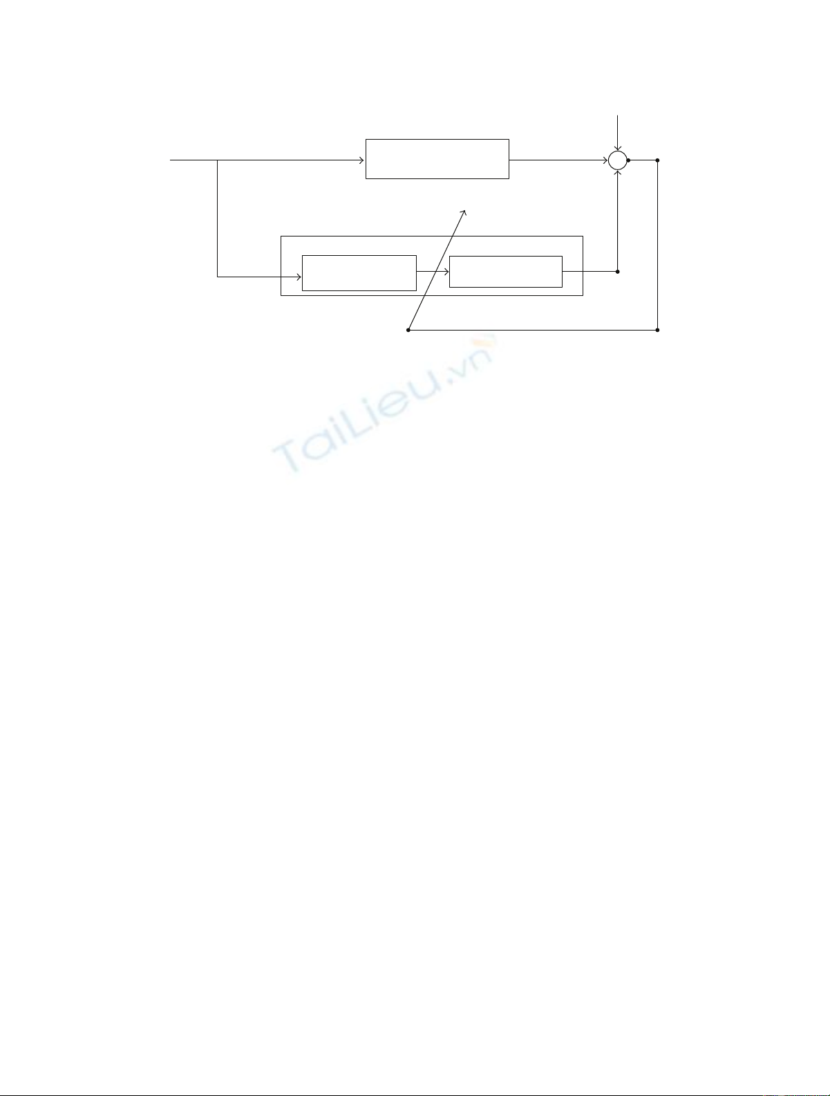
This work will focus on the Hammerstein nonlinear system
depicted in Figure 1. Hammerstein nonlinear models have
been applied to modeling distortion in nonlinearly ampli-
fied digital communication signals (satellite and microwave
links) followed by a linear channel [5,6]. In the area
of biomedical engineering, the Hammerstein model finds
application in modeling the involuntary contraction of
human muscles [7,8] and human heart rate regulation
during treadmill exercise [9]. Hammerstein systems are also
applied in the area of Neural Network since it provides
a convenient way to deal with nonlinearity [10]. Existing
Hammerstein nonlinear system identification techniques can
be divided into three groups:
(i) deterministic techniques such as orthogonal least-
squares expansion method [11–13],
(ii) stochastic techniques based on recursive algorithms
[14,15] or nonadaptive methods [16], and
(iii) adaptive techniques [17–20].
Adaptive Hammerstein algorithms have been achieved
using block based adaptive algorithms [11,20]. In block
based adaptive Hammerstein algorithms, the Hammerstein
system is overparameterized in such a way that the Ham-
merstein system is linear in the unknown parameters. This
allows the use of any linear estimation algorithm in solving
the Hammerstein nonlinear system identification problem.
The limitation of this approach is that the dimension
of the resulting linear block system can be very large,
and therefore, convergence or robustness of the algorithm
becomes an issue [18]. Recently, Bai reported a blind
approach to Hammerstein system identification using least
mean square (LMS) algorithm [18]. The method reported
applied a two-stage identification process (Linear Infinite
Impulse Response (IIR) stage and the nonlinear stage)
without any knowledge of the internal signals connecting
both cascades in the Hammerstein system. This method
requires a white input signal to guarantee the stability
and convergence of the algorithm. Jeraj and Mathews
derived an adaptive Hammerstein system identification
algorithm by linearizing the system nonlinearity using a
Gram-Schmidt orthogonalizer at the input to the linear
subsystem (forming an MISO system) [17]. This method
also suffers the same limitations as the block-based adaptive
Hammerstein algorithms. Thus, to improve the speed of
2 EURASIP Journal on Advances in Signal Processing
Polynomial nonlinearity
Hammerstein nonlinear filter
Infinite impulse
response filter
d(n)
x(n) e(n)
v(n)
Plant (unknown system)
d(n)
z(n)
Figure 1: Adaptive system identification of a Hammerstein system model.
convergence while maintaining a small misadjustment and
computational complexity, the Affine Projection theory is
used as opposed to LMS [18] or Recursive Least squares
(RLSs).
In nonlinear system identification, input signals with
high eigen value spread, ill-conditioned tap input autocorre-
lation matrix can lead to divergence or poor performance of a
fixed step-size adaptive algorithm. To mitigate this problem,
a number of variable step-size update algorithms have been
proposed. These variable step-size update algorithms can
be roughly divided into gradient adaptive step-size [21,
22] and normalized generalized gradient descent [23]. The
major limitation of gradient adaptive step-size algorithms
is their sensitivity to the time correlation between input
signal samples and the value of the additional step-size
parameter that governs the gradient adaptation of the
step-size. As a result of these limitations, a criteria for
the choice of the step-size based on Lyapunov stability
theory is proposed to track the optimal step-size required
to maintain a fast convergence rate and low misadjust-
ment.
In this paper, we focus on the adaptive system identifi-
cation problem of a class of Hammerstein output error type
nonlinear systems with polynomial nonlinearity. Our unique
contributions in the paper are as follows.
(1) Using the theory of affine projections [24], we derive
an adaptive Hammerstein algorithm that identifies
the linear subsystem of the Hammerstein system
without prior knowledge of the input signal z(n).
(2) Employing the Lyapunov stability theory, we develop
criteria for the choice of the algorithms step-size
which ensures the minimization of the Lyapunov
function. This is particularly important for the
stability of the linear algorithm regardless of the
location of the poles of the IIR filter.
Briefly, the paper is organized as follows. Section 2
describes the nonlinear Hammerstein system identifica-
tion problem addressed in this paper. Section 3 contains
a detailed derivation of the proposed variable step-size
adaptive Hammerstein algorithm. Section 4 provides both
a hypothetical and real life data simulation validating the
effectiveness of the variable step-size adaptive algorithm
proposed. Finally, we conclude with a brief summary in
Section 5.
2. Problem Statement
Consider the Hammerstein model shown in Figure 1,where
x(n), v(n), and
d(n) are the systems input, noise, and output,
respectively. z(n) represents the unavailable internal signal
output of the memoryless polynomial nonlinear system.
The output of the memoryless polynomial nonlinear system,
which is the input to the linear system, is given by
z(n)=
L
l=1
pl(n)xl(n).(1)
Let the discrete linear time-invariant system be an infinite
impulse response (IIR) filter satisfying a linear difference
equation of the form
d(n)=−
N
i=1
ai(n)
d(n−i)+
M
j=0
bj(n)zn−j,(2)
where pl(n), ai(n), and bj(n) represent the coefficients of
the nonlinear Hammerstein system at any given time n.To
ensure uniqueness, we set b0(n)=1 (any other coefficient
other than b0(n)canbesetto1).Thus,(2)canbewrittenas
d(n)=
L
l=1
pl(n)xl(n)−
N
i=1
ai(n)
d(n−i)+
M
j=1
bj(n)zn−j.
(3)

EURASIP Journal on Advances in Signal Processing 3
Let
θ(n)=[a1(n)··· aN(n)b1(n)··· bM(n)
p1(n)··· pL(n)H,
b0=1,
s(n)=−
d(n−1)··· −
d(n−N)
z(n−1)··· z(n−M)
x(n)··· xL(n)H.
(4)
Equation (3) can be rewritten in compact form
d(n)=s(n)H
θ(n).(5)
The goal of the Adaptive nonlinear Hammerstein system
identification is to estimate the coefficient vector (
θ(n)) in
(5) of the nonlinear Hammerstein filter based only on the
input signal x(n)andoutputsignald(n) such that
d(n)is
close to the desired response signal d(n).
3. Adaptive Hammerstein Algorithm
In this section, we develop an algorithm based on the theory
of Affine projection [24] for estimation of the coefficients
of the nonlinear Hammerstein system using the plant input
and output signals. The main idea of our approach to
nonlinear Hammerstein system identification is to formulate
a criterion for designing a variable step-size affine projection
Hammerstein filter algorithm and then use the criterion in
minimizing the cost function.
3.1. Stochastic Gradient Minimization Approach. We formu-
late the criterion for designing the adaptive Hammerstein
filter as the minimization of the square Euclidean norm of
the change in the weight vector
θ(n)=
θ(n)−
θ(n−1)(6)
subject to the set of Qconstraints
dn−q=sn−qH
θ(n)q=1, ...,Q. (7)
Applying the method of Lagrange multipliers with
multiple constraints to (6)and(7), the cost function for the
affine projection filter is written as (assuming real data)
J(n−1)=
θ(n)−
θ(n−1)
2+Re
[(n−1)λ],(8)
where
(n−1)=d(n−1)−
S(n−1)H
θ(n),
d(n−1)=[d(n−1)··· d(n−Q)]H,
S(n−1)=[s(n−1)··· s(n−Q)],
λ=λ1··· λQH.
(9)
Minimizing the cost function (8) (squared prediction
error) with respect to the nonlinear Hammerstein filter
weight vector
θ(n)gives
∂J(n−1)
∂
θ(n)=2
θ(n)−
θ(n−1)−∂
θ(n)H
S(n−1)λ
∂
θ(n),
(10)
where
∂
θ(n)H
S(n−1)
∂
θ(n)
=∂
θ(n)Hs(n−1)
∂
θ(n)··· ∂
θ(n)Hs(n−Q)
∂
θ(n).
(11)
Since a portion of the vectors s(n)in
S(n) include past
d(n) which are dependent on past
θ(n) which are used to
form the new
θ(n), the partial derivative of each element in
(10)gives
∂
θ(n)Hsn−q
∂ai(n)=−
dn−q−i−
N
k=1
ak(n)∂
dn−q−k
∂ai(n),
(12)
∂
θ(n)Hsn−q
∂bj(n)=zn−q−j−
N
k=1
ak(n)∂
dn−q−k
∂bj(n),
(13)
∂
θ(n)Hsn−q
∂pl(n)=xln−q+
M
k=1
bk(n)∂zn−q−k
∂pl(n)
−
N
k=1
ak(n)∂
dn−q−k
∂pl(n).
(14)
From (12), (13), and (14) it is necessary to evaluate
the derivative of past
d(n)withrespecttocurrentweight
estimates. In evaluating the derivative of
d(n)withrespect
to the current weight vector, we assume that the step-size of
the adaptive algorithm is chosen such that [24]
θ(n)∼
=
θ(n−1)∼
=···∼
=
θ(n−N).(15)
Therefore
ai(n)∼
=ai(n−1)∼
=···∼
=ai(n−N),
∂
dn−q
∂ai(n)=−
dn−q−i−
N
k=1
ak(n)∂
dn−q−k
∂ai(n−k)
bj(n)∼
=bj(n−1)∼
=···∼
=bj(n−N),
,
(16)

4 EURASIP Journal on Advances in Signal Processing
∂
dn−q
∂bj(n)=zn−q−j−
N
k=1
ak(n)∂
dn−q−k
∂bj(n−k),
pl(n)∼
=pl(n−1)∼
=···∼
=pl(n−N),
(17)
∂
dn−q
∂pl(n)=xln−q+
M
k=1
bk(n)∂zn−q−k
∂pl(n−k).
−
N
k=1
ak(n)∂
dn−q−k
∂pl(n−k),
(18)
∂pln−q−k
∂pl(n−k)=1, (19)
thus,
∂
dn−q
∂pl(n)=xln−q+
M
k=1
bk(n)xln−q−k
−
N
k=1
ak(n)∂
dn−q−k
∂pl(n−k),
(20)
where
φn−q=∂
dn−q
∂
θ(n)
=⎡
⎣∂
dn−q
∂a1(n)··· ∂
dn−q
∂aN(n)
∂
dn−q
∂b1(n)
··· ∂
dn−q
∂bM(n)
∂
dn−q
∂p1(n)··· ∂
dn−q
∂pL(n)⎤
⎦
H
.
(21)
Let
Φ(n−1)=∂
θ(n)H
S(n−1)
∂
θ(n),
ψn−q=−
dn−q−1··· −
dn−q−N
zn−q−1
···
zn−q−MM
j=0
xn−q−j
···
M
j=0
xLn−q−j⎤
⎦
H
,
Ψ(n−1)=
ψ(n−1)···
ψ(n−Q).
(22)
Substituting (16), (17), and (20) into (11), we get
Φ(n−1)=
Ψ(n−1)−
N
k=1
ak(n−1)
Φ(n−1−k).(23)
Thus, rewriting (10)
∂J(n−1)
∂
θ(n)=2
θ(n)−
θ(n−1)−
Φ(n−1)λ. (24)
Setting the partial derivative of the cost function in (24)to
zero, we get
θ(n)=1
2
Φ(n−1)λ. (25)
From (7), we can write
d(n−1)=
S(n−1)H
θ(n), (26)
where
d(n−1)=[d(n−1)··· d(n−Q)],
d(n−1)=
S(n−1)H
θ(n−1)+1
2
S(n−1)H
Φ(n−1)λ.
(27)
Evaluating (27)forλresults in
λ=2
S(n−1)H
Φ(n−1)−1e(n−1), (28)
where
e(n−1)=d(n−1)−
S(n−1)H
θ(n−1).(29)
Substituting (28) into (25) yields the optimum change in
the weight vector
θ(n)=
Φ(n−1)
S(n−1)H
Φ(n−1)−1e(n−1).(30)
Assuming that the input to the linear part of the
nonlinear Hammerstein filter is a memoryless polynomial
nonlinearity, we normalize (30)asin[25] and exercise con-
trol over the change in the weight vector from one iteration to
the next keeping the same direction by introducing the step-
size μ. Regularization of the
S(n−1)H
Φ(n−1) matrix is also
used to guard against numerical difficulties during inversion,
thus yielding
θ(n)=
θ(n−1)−μ
Φ(n−1)
×
ΦδI +μ
S(n−1)H(n−1)−1e(n−1).
(31)
To improve the update process Newton’s method is applied
by scaling the update vector by R−1(n). The matrix R(n)is
recursively computed as
R(n)=λnR(n−1)+(1−λn)
Φ(n−1)
Φ(n−1)H, (32)
where λnis typically chosen between 0.95 and 0.99. Applying
the matrix inversion lemma on (32) and using the result in
(31), the new update equation is given by
θ(n)=
θ(n−1)−μR(n−1)−1
Φ(n−1)
×δI +μ
S(n−1)H
Φ(n−1)−1e(n−1)
(33)

EURASIP Journal on Advances in Signal Processing 5
3.2. Variable Step-Size. In this subsection, we derive an
update for the step-size using a Lyapunov function of
summed squared nonlinear Hammerstein filter weight esti-
mate error. The variable step-size derived guarantees the
stable operation of the linear IIR filter by satisfying the
stability condition for the choice of μin [26]. Let
θ(n)=θ−
θ(n), (34)
where θrepresents the optimum Hammerstein system
coefficient vector. We propose the Lyapunov function V(n)
as
V(n)=θ(n)Hθ(n), (35)
which is the general form of the quadratic Lyapunov function
[27]. The Lyapunov function is positive definite in a range
of values close to the optimum θ=
θ(n). In order for
the multidimensional error surface to be concave, the time
derivative of the Lyapunov function must be semidefinite.
This implies that
ΔV(n)=V(n)−V(n−1)≤0.(36)
From the Hammerstein filter update equation
θ(n)=
θ(n−1)−μ
Φ(n−1)
S(n−1)H
Φ(n−1)−1e(n−1),
(37)
we subtract θfrom both sides to yeild
θ(n)=θ(n−1)−μ
Φ(n−1)
S(n−1)H
Φ(n−1)−1e(n−1).
(38)
From (35), (36), and (38)wehave
ΔV(n)=θ(n)Hθ(n)−θ(n−1)Hθ(n−1).(39)
Minimizing the Lyapunov function with respect to the
step-size μ, and equating the result to zero, we obtain the
optimum value for μas μopt
μopt =
Eθ(n−1)H
Φ(n−1)
S(n−1)H
Φ(n−1)−1e(n−1)
Ee(n−1)HΥ(n−1)HΥ(n−1)e(n−1),
(40)
where
Υ(n−1)=
Φ(n−1)
S(n−1)H
Φ(n−1)−1.(41)
Adding the system noise v(n) to the desired output and
assuming that the noise is independently and identically
distributed and statistically independent of
S(n), we have
d(n)=
S(n)Hθ+v(n).(42)
INITIALIZE: R−1(0) =I,λn/
=0, 0 <β≤1
for n=0 to sample size do
e(n−1) =d(n−1) −
S(n−1)H
θ(n−1)
Φ(n−1) =
Ψ(n−1) −N
k=1ak(n−1)
Φ(n−1−k)
B(n)=α
B(n−1) −(1 −α)Υ(n−1)e(n−1)
μ(n)=
μopt(
B(n)2
B(n)2+C
)
(λn
1−λn
I−
Φ(n−1)HR(n−1)−1
Φ(n−1))−1
R(n)−1=1
λn
[R(n−1)−1−R(n−1)−1
Φ(n−1)
Φ(n−1)HR(n−1)−1]
θ(n)=
θ(n−1) −μ(n)R(n)−1
Φ(n−1)
(δI +μ(n)
S(n−1)H
Φ(n−1))−1e(n−1)
z(n)=x(n)Hp(n)
d(n)=
s(n)H
θ(n)
end for
Algorithm 1: Summary of the proposed Variable Step-size Ham-
merstein adaptive algorithm.
From (40)wewrite
μoptEe(n−1)HΥ(n−1)HΥ(n−1)e(n−1)
=Eθ(n−1)H
Φ(n−1)
S(n−1)H
Φ(n−1)−1e(n−1).
(43)
The computation of μopt requires the knowledge of θ(n−1)
which is not available during adaptation. Thus, we propose
the following suboptimal estimate for μ(n):
μ(n)=
μoptEΥ(n−1)e(n−1)2
EΥ(n−1)e(n−1)2+σ2
vTrEΥ(n−1)2.
(44)
We estimate EΥ(n−1)e(n−1)by time averaging as follows:
B(n)=α
B(n−1)−(1−α)Υ(n−1)e(n−1)
μ(n)=μopt⎛
⎜
⎝
B(n)
2
B(n)
2+C⎞
⎟
⎠,(45)
where μopt is an rough estimate of μopt,αis a smoothing
factor (0 <α<1), and Cis a constant representing
σ2
vTr{Υ(n−1)2}≈Q/SNR. We guarantee the stability of
the Hammerstein filter by choosing μopt to satisfy the stability
bound in [26]. Choosing μopt to satisfy the stability bound
[26] will bound the step-size update μ(n) with an upper limit
of μopt thereby ensuring the slow variation and stability of the
linear IIR filter.
A summary of the proposed algorithm is shown in
Algorithm 1. In the algorithm, Nrepresents the number


![Báo cáo seminar chuyên ngành Công nghệ hóa học và thực phẩm [Mới nhất]](https://cdn.tailieu.vn/images/document/thumbnail/2025/20250711/hienkelvinzoi@gmail.com/135x160/47051752458701.jpg)


%20--%3e%3cdefs%3e%3cstyle%3e%20.st0%20{%20fill:%20%23fff;%20}%20.st1%20{%20fill:%20%237800fa;%20}%20%3c/style%3e%3c/defs%3e%3cpath%20class='st1'%20d='M117.78,12.18H43.11c2.9,3.47,4.65,7.94,4.65,12.82,0,5.6-2.3,10.66-6.01,14.29h76.02l7.22-13.56-7.22-13.56Z'/%3e%3cg%3e%3cpath%20class='st0'%20d='M53.58,26.17h-.59v-1.46h.59v-4.96h2.83c1.78,0,2.67.94,2.67,2.82v5.76c0,1.87-.89,2.81-2.67,2.81h-2.83v-4.96ZM55.36,21.37v3.34h1.1v1.46h-1.1v3.34h1.01c.61,0,.91-.37.91-1.1v-5.93c0-.74-.3-1.1-.91-1.1h-1.01Z'/%3e%3cpath%20class='st0'%20d='M65.99,31.14h-1.8l-.31-2.07h-2.19l-.31,2.07h-1.64l1.82-11.39h2.62l1.82,11.39ZM65.28,18.04c-.25.46-.51.77-.75.94-.21.15-.47.22-.79.22-.26,0-.57-.07-.92-.22l-.38-.15c-.14-.05-.26-.07-.37-.07-.3,0-.53.18-.71.54l-.91-.68c.25-.46.51-.77.75-.94.21-.14.48-.21.79-.21.26,0,.57.07.92.21l.38.15c.14.05.26.07.37.07.3,0,.53-.18.71-.54l.91.68ZM61.91,27.52h1.73l-.87-5.76-.87,5.76Z'/%3e%3cpath%20class='st0'%20d='M74.53,26.89v1.52c0,1.91-.89,2.86-2.67,2.86s-2.67-.95-2.67-2.86v-5.93c0-1.91.89-2.86,2.67-2.86s2.67.95,2.67,2.86v1.11h-1.69v-1.22c0-.75-.31-1.12-.93-1.12s-.93.37-.93,1.12v6.15c0,.74.31,1.11.93,1.11s.93-.37.93-1.11v-1.63h1.69Z'/%3e%3cpath%20class='st0'%20d='M81.4,31.14h-1.8l-.31-2.07h-2.19l-.31,2.07h-1.64l1.82-11.39h2.62l1.82,11.39ZM75.9,19.2l1.52-1.91h1.71l1.51,1.91h-1.61l-.76-.95-.75.95h-1.61ZM77.32,27.52h1.73l-.87-5.76-.87,5.76ZM83.1,15.99l-1.76,1.91h-1.26l1.17-1.91h1.86Z'/%3e%3cpath%20class='st0'%20d='M84.86,19.75c1.78,0,2.67.94,2.67,2.82v1.48c0,1.87-.89,2.81-2.67,2.81h-.85v4.28h-1.79v-11.39h2.64ZM84.01,21.37v3.86h.85c.58,0,.87-.36.87-1.08v-1.71c0-.71-.29-1.07-.87-1.07h-.85Z'/%3e%3cpath%20class='st0'%20d='M93.51,19.75c1.78,0,2.67.94,2.67,2.82v1.48c0,1.87-.89,2.81-2.67,2.81h-.85v4.28h-1.79v-11.39h2.64ZM92.66,21.37v3.86h.85c.58,0,.87-.36.87-1.08v-1.71c0-.71-.29-1.07-.87-1.07h-.85Z'/%3e%3cpath%20class='st0'%20d='M98.8,31.14h-1.79v-11.39h1.79v4.88h2.03v-4.88h1.83v11.39h-1.83v-4.88h-2.03v4.88Z'/%3e%3cpath%20class='st0'%20d='M105.36,24.55h2.46v1.62h-2.46v3.34h3.09v1.63h-4.88v-11.39h4.88v1.63h-3.09v3.18ZM108.17,17.29l-1.76,1.91h-1.26l1.17-1.91h1.86Z'/%3e%3cpath%20class='st0'%20d='M112.2,19.75c1.78,0,2.67.94,2.67,2.82v1.48c0,1.87-.89,2.81-2.67,2.81h-.85v4.28h-1.79v-11.39h2.64ZM111.35,21.37v3.86h.85c.58,0,.87-.36.87-1.08v-1.71c0-.71-.29-1.07-.87-1.07h-.85Z'/%3e%3c/g%3e%3ccircle%20class='st1'%20cx='25'%20cy='25'%20r='20'/%3e%3cpath%20class='st0'%20d='M32.78,19.27c2.92,0,4.43,2.55,5.28,5.33l.71,2.17c.14.38-.33.75-.71.75h-5.61c.19-.33.24-.71.09-1.08l-.75-2.45c-.43-1.32-.99-2.64-1.79-3.77.75-.57,1.65-.94,2.78-.94h0ZM25,18.38c3.25,0,4.9,2.78,5.89,5.89l.76,2.45c.14.42-.33.8-.8.8h-11.69c-.42,0-.94-.38-.8-.8l.75-2.45c.99-3.11,2.64-5.89,5.89-5.89h0ZM25,11.35c1.74,0,3.11,1.37,3.11,3.11s-1.37,3.11-3.11,3.11-3.11-1.41-3.11-3.11,1.41-3.11,3.11-3.11h0ZM17.27,19.27c1.08,0,1.98.38,2.73.94-.8,1.13-1.37,2.45-1.74,3.77l-.8,2.45c-.14.38-.05.75.09,1.08h-5.56c-.42,0-.9-.38-.75-.75l.71-2.17c.9-2.78,2.41-5.33,5.33-5.33h0ZM17.27,12.91c1.51,0,2.78,1.27,2.78,2.83s-1.27,2.83-2.78,2.83-2.83-1.27-2.83-2.83,1.27-2.83,2.83-2.83h0ZM32.78,12.91c1.56,0,2.78,1.27,2.78,2.83s-1.23,2.83-2.78,2.83-2.83-1.27-2.83-2.83,1.27-2.83,2.83-2.83h0ZM27.07,28.56v.09c0,.57-.24,1.08-.61,1.46h0v.05c-.38.33-.9.57-1.46.57s-1.08-.24-1.46-.61h0c-.38-.38-.61-.9-.61-1.46v-.09h1.41v.09c0,.19.05.38.19.47v.05c.09.09.28.19.47.19s.38-.09.47-.19v-.05c.14-.09.24-.28.24-.47t-.05-.09h1.41ZM30.99,28.56v.09c0,1.65-.66,3.16-1.74,4.24-1.08,1.08-2.59,1.79-4.24,1.79s-3.16-.71-4.24-1.79l-.05-.05c-1.04-1.08-1.7-2.55-1.7-4.2v-.09h1.41v.09c0,1.27.47,2.4,1.27,3.25h.05c.85.85,1.98,1.37,3.25,1.37s2.4-.52,3.25-1.37c.85-.8,1.37-1.98,1.37-3.25v-.09h1.37ZM34.99,28.56v.09c0,2.78-1.13,5.28-2.92,7.07-1.79,1.79-4.29,2.92-7.07,2.92s-5.23-1.13-7.07-2.92c-1.79-1.79-2.92-4.29-2.92-7.07v-.09h1.41v.09c0,2.4.94,4.53,2.5,6.08,1.56,1.56,3.72,2.5,6.08,2.5s4.52-.94,6.08-2.5c1.56-1.56,2.5-3.68,2.5-6.08v-.09h1.41Z'/%3e%3c/svg%3e)