Bài giảng Tối ưu hóa nâng cao: Chương 5

Gradient Descent

Hoàng Nam Dũng

Khoa Toán - Cơ - Tin học, Đại học Khoa học Tự nhiên, Đại học Quốc gia Hà Nội

Gradient descent: choose initial point x (0) Rn, repeat: ∈ f (x (k−1)), k = 1, 2, 3, . . . x (k) = x (k−1) tk − · ∇ Stop at some point.

Gradient descent

Consider unconstrained, smooth convex optimization

f (x) min x R. Denote the optimal → with convex and differentiable function f : Rn value by f ∗ = minx f (x) and a solution by x ∗.

Gradient descent

Consider unconstrained, smooth convex optimization

f (x) min x R. Denote the optimal → with convex and differentiable function f : Rn value by f ∗ = minx f (x) and a solution by x ∗.

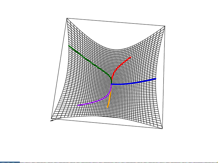
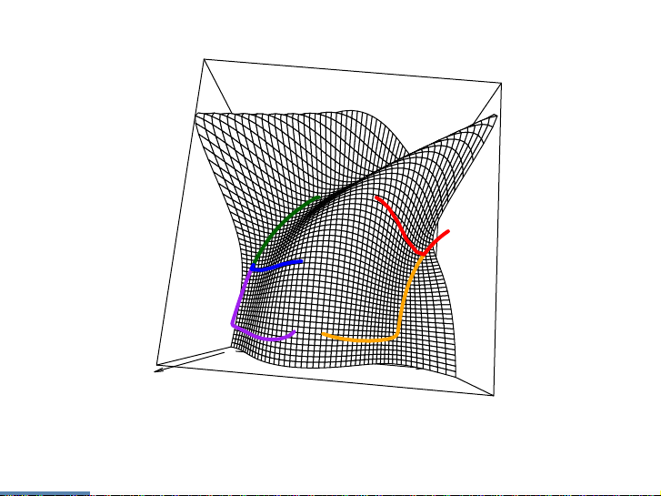
Gradient descent: choose initial point x (0) Rn, repeat:

∈ f (x (k−1)), k = 1, 2, 3, . . . x (k) = x (k−1) tk − · ∇ Stop at some point.

Gradient descent interpretation

At each iteration, consider the expansion

x f (y ) f (x) + f (x)T (y x) + ≈ ∇ − 1 y 2t (cid:107)

2 2 . − (cid:107) 2f (x) by 1

t I .

Quadratic approximation, replacing usual Hessian ∇ x) − linear approximation to f proximity term to x, with weight 1/2t f (x) + ∇ 1 2t (cid:107) f (x)T (y 2 x y 2 (cid:107) −

t Choose next point y = x + to minimize quadratic approximation x + = x f (x). − ∇

Gradient descent interpretation

Blue point is x, red point is

x ∗ = argminy f (x) + ∇f (x)T (y − x) + 1

2t (cid:107)y − x(cid:107)2

Outline

(cid:73) How to choose step sizes

(cid:73) Convergence analysis

(cid:73) Nonconvex functions

(cid:73) Gradient boosting

Fixed step size

2 )/2, gradient descent after 8 steps:

1 + x 2

Simply take tk = t for all k = 1, 2, 3, . . ., can diverge if t is too big. Consider f (x) = (10x 2

Fixed step size

Can be slow if t is too small. Same example, gradient descent after 100 steps:

Fixed step size

Converges nicely when t is “just right”. Same example, 40 steps:

Convergence analysis later will give us a precise idea of “just right”.

Backtracking line search

(cid:73) First fix parameters 0 < β < 1 and 0 < α

One way to adaptively choose the step size is to use backtracking line search:

(cid:73) At each iteration, start with t = tinit, and while

1/2. ≤

2 2

t f (x)) > f (x) f (x αt (cid:107)∇ ∇ − − f (x) (cid:107) shrink t = βt. Else perform gradient descent update

t x + = x f (x). − ∇

Simple and tends to work well in practice (further simplification: just take α = 1/2).

Backtracking interpretation

For us ∆x = −∇f (x)

Backtracking line search

Setting α = β = 0.5, backtracking picks up roughly the right step size (12 outer steps, 40 steps total).

Exact line search

We could also choose step to do the best we can along direction of negative gradient, called exact line search:

s f (x)). t = argmins≥0 f (x − ∇ Usually not possible to do this minimization exactly.

Approximations to exact line search are typically not as efficient as backtracking and it’s typically not worth it.

We say gradient descent has convergence rate O(1/k), i.e., it finds ε-suboptimal point in O(1/ε) iterations.

Chứng minh.

Slide 20-25 in http://www.seas.ucla.edu/~vandenbe/236C/ lectures/gradient.pdf

Convergence analysis

R convex and differentiable and additionally → L y Assume that f : Rn f (x) f (y ) for any x, y (cid:107)∇ (cid:107)2 ≤ x (cid:107) (cid:107)2 − − ∇ i.e., f is Lipschitz continuous with constant L > 0.

∇ Theorem

2 2 (cid:107)

1/L satisfies ≤ f ∗ x (0) x ∗ f (x (k)) Gradient descent with fixed step size t 1 2tk (cid:107) ≤ − − and same result holds for backtracking with t replaced by β/L.

Chứng minh.

Slide 20-25 in http://www.seas.ucla.edu/~vandenbe/236C/ lectures/gradient.pdf

Convergence analysis

∇ Theorem

2 2 (cid:107)

1/L satisfies ≤ f ∗ x (0) x ∗ f (x (k)) Gradient descent with fixed step size t 1 2tk (cid:107) − ≤ − and same result holds for backtracking with t replaced by β/L.

We say gradient descent has convergence rate O(1/k), i.e., it finds ε-suboptimal point in O(1/ε) iterations.

Convergence analysis

∇ Theorem

2 2 (cid:107)

1/L satisfies ≤ f ∗ x (0) x ∗ f (x (k)) Gradient descent with fixed step size t 1 2tk (cid:107) ≤ − − and same result holds for backtracking with t replaced by β/L.

We say gradient descent has convergence rate O(1/k), i.e., it finds ε-suboptimal point in O(1/ε) iterations.

Chứng minh.

Slide 20-25 in http://www.seas.ucla.edu/~vandenbe/236C/ lectures/gradient.pdf

Rate under strong convexity is O(c k ), exponentially fast, i.e., we find ε-suboptimal point in O(log(1/ε)) iterations.

Chứng minh.

Slide 26-27 in http://www.seas.ucla.edu/~vandenbe/236C/ lectures/gradient.pdf

Convergence under strong convexity

m 2 (cid:107)

2 2 is convex for some (cid:107)

x − Reminder: strong convexity of f means f (x) m > 0.

Assuming Lipschitz gradient as before and also strong convexity:

Theorem

2/(m + L) or with backtracking Gradient descent with fixed step size t line search search satisfies

2 2

f ∗ x ∗ x (0) f (x (k)) − ≤ (cid:107) − ≤ c k L 2 (cid:107) where 0 < c < 1.

Chứng minh.

Slide 26-27 in http://www.seas.ucla.edu/~vandenbe/236C/ lectures/gradient.pdf

Convergence under strong convexity

m 2 (cid:107)

2 2 is convex for some (cid:107)

x − Reminder: strong convexity of f means f (x) m > 0.

Assuming Lipschitz gradient as before and also strong convexity:

Theorem

2/(m + L) or with backtracking Gradient descent with fixed step size t line search search satisfies

2 2

f ∗ x ∗ x (0) f (x (k)) − ≤ (cid:107) − ≤ c k L 2 (cid:107) where 0 < c < 1.

Rate under strong convexity is O(c k ), exponentially fast, i.e., we find ε-suboptimal point in O(log(1/ε)) iterations.

Convergence under strong convexity

m 2 (cid:107)

2 2 is convex for some (cid:107)

x − Reminder: strong convexity of f means f (x) m > 0.

Assuming Lipschitz gradient as before and also strong convexity:

Theorem

2/(m + L) or with backtracking Gradient descent with fixed step size t line search search satisfies

2 2

f ∗ x ∗ x (0) f (x (k)) − ≤ (cid:107) − ≤ c k L 2 (cid:107) where 0 < c < 1.

Rate under strong convexity is O(c k ), exponentially fast, i.e., we find ε-suboptimal point in O(log(1/ε)) iterations.

Chứng minh.

Slide 26-27 in http://www.seas.ucla.edu/~vandenbe/236C/ lectures/gradient.pdf

Convergence rate

(From B & V page 487)

Called linear convergence, because looks linear on a semi-log plot.

slower rate. Important note: contraction factor c in rate depends adversely on condition number L/m: higher condition number ⇒

Affects not only our upper bound. . . very apparent in practice too.

A look at the conditions

2 2. (cid:107)

A look at the conditions for a simple problem, f (β) = 1 X β y 2 (cid:107) −

(cid:73) This mean

2f (x)

(cid:73) As

2f (β) = X T X , we have L = σmax(X T X ).

Lipschitz continuity of f : ∇ LI . ∇ (cid:22)

(cid:73) This mean

∇ Strong convexity of f :

2f (x)

(cid:73) As

2f (β) = X T X , we have m = σmin(X T X ).

mI . ∇ (cid:23)

(cid:73) If X is wide (i.e., X is n

(cid:73) Even if σmin(X T X ) > 0, can have a very large condition number

∇ p with p > n), then σmin(X T X ) = 0, and × f can’t be strongly convex.

L/m = σmax(X T X )/σmin(X T X ).

(cid:73) Pro: simple idea, and each iteration is cheap (usually)

(cid:73) Pro: fast for well-conditioned, strongly convex problems

(cid:73) Con: can often be slow, because many interesting problems aren’t

Pros and cons of gradient descent:

(cid:73) Con: can’t handle nondifferentiable functions.

strongly convex or well-conditioned

Practicalities

(cid:73) Recall

(cid:73) If f is strongly convex with parameter m, then

Stopping rule: stop when f (x) (cid:107)2 is small (cid:107)∇ f (x ∗) = 0 at solution x ∗ ∇

f ∗ f (x) √2mε = f (x) ε. (cid:107)∇ (cid:107)2 ≤ ⇒ − ≤

Practicalities

(cid:73) Recall

(cid:73) If f is strongly convex with parameter m, then

Stopping rule: stop when f (x) (cid:107)2 is small (cid:107)∇ f (x ∗) = 0 at solution x ∗ ∇

(cid:73) Pro: simple idea, and each iteration is cheap (usually)

(cid:73) Pro: fast for well-conditioned, strongly convex problems

(cid:73) Con: can often be slow, because many interesting problems aren’t

f ∗ f (x) √2mε = f (x) ε. (cid:107)∇ (cid:107)2 ≤ ⇒ − ≤ Pros and cons of gradient descent:

(cid:73) Con: can’t handle nondifferentiable functions.

strongly convex or well-conditioned

Theorem (Nesterov)

For any k (n 1)/2 and any starting point x (0), there is a function f ≤ − in the problem class such that any first-order method satisfies

3L (cid:13) x ∗(cid:13) (cid:13)x (0) (cid:13) − f ∗ f (x (k)) . 32(k + 1)2 − ≥

Can attain rate O(1/k 2), or O(1/√ε)? Answer: yes (we’ll see)!

Can we do better?

Gradient descent has O(1/ε) convergence rate over problem class of convex, differentiable functions with Lipschitz gradients.

First-order method: iterative method, which updates x (k) in f (x (k−1)) f (x (0)), f (x (1)), . . . , x (0) + span {∇ ∇ ∇ . }

Can we do better?

Gradient descent has O(1/ε) convergence rate over problem class of convex, differentiable functions with Lipschitz gradients.

First-order method: iterative method, which updates x (k) in f (x (k−1)) f (x (0)), f (x (1)), . . . , x (0) + span {∇ ∇ ∇ . }

Theorem (Nesterov)

1)/2 and any starting point x (0), there is a function f (n ≤ − For any k in the problem class such that any first-order method satisfies

3L (cid:13) − f ∗ . f (x (k)) x ∗(cid:13) 2 (cid:13)x (0) (cid:13) 2 32(k + 1)2 − ≥

Can attain rate O(1/k 2), or O(1/√ε)? Answer: yes (we’ll see)!

Theorem

i=0,...,k (cid:107)∇

Gradient descent with fixed step size t 1/L satisfies ≤ (cid:115) 2(f (x 0) f ∗) min f (x (i)) . − t(k + 1) (cid:107) ≤

Thus gradient descent has rate O(1/√k), or O(1/ε2), even in the nonconvex case for finding stationary points.

This rate cannot be improved (over class of differentiable functions with Lipschitz gradients) by any deterministic algorithm1.

What about nonconvex functions?

1Carmon et al. (2017), “Lower bounds for finding stationary points I”

Assume f is differentiable with Lipschitz gradient as before, but now nonconvex. Asking for optimality is too much. So we’ll settle for x such that ε, called ε-stationarity. f (x) (cid:107)∇ (cid:107)2 ≤

What about nonconvex functions?

i=0,...,k (cid:107)∇

2 (cid:107)

Gradient descent with fixed step size t 1/L satisfies ≤ (cid:115) 2(f (x 0) f ∗) min f (x (i)) . − t(k + 1) ≤

Thus gradient descent has rate O(1/√k), or O(1/ε2), even in the nonconvex case for finding stationary points.

1Carmon et al. (2017), “Lower bounds for finding stationary points I”

This rate cannot be improved (over class of differentiable functions with Lipschitz gradients) by any deterministic algorithm1.

Proof

(cid:73)

Key steps:

2 2 , (cid:107)

2 2 .

(cid:73) Taking 0 < t

2 2 ≤ (cid:107)

(cid:73) Summing over iterations

k (cid:88)

f Lipschitz with constant L means ∇ y x f (y ) f (x) + f (x)T (y x) + x, y . L 2 (cid:107) − ≤ ∀ t ∇ (cid:73) Plugging in y = x + = x ∇ − f (x), (cid:18) (cid:19) 1 t − f (x) f (x +) Lt 2 ≤ − f (x) (cid:107) (cid:107)∇ − 1/L, and rearranging, ≤ (f (x) f (x +)). f (x) 2 t − (cid:107)∇

2 ≤

i=0

(f (x (0)) f (x (k+1))) (f (x (0)) f ∗). (cid:13) 2 f (x (i)) (cid:13) (cid:13) 2 t 2 t (cid:13) (cid:13) (cid:13)∇ ≤ − −

(cid:73) Lower bound sum by (k + 1) mini=0,1,...

f (x (i)) (cid:13) (cid:13) (cid:13) 2 2, conclude. (cid:13) ∇

References and further reading

S. Boyd and L. Vandenberghe (2004), Convex optimization, Chapter 9

T. Hastie, R. Tibshirani and J. Friedman (2009), The elements of statistical learning, Chapters 10 and 16

Y. Nesterov (1998), Introductory lectures on convex optimization: a basic course, Chapter 1

L. Vandenberghe, Lecture notes for EE 236C, UCLA, Spring 2011-2012

Bài giảng Tối ưu hóa nâng cao: Chương 5 - Hoàng Nam Dũng