Bài giảng Tối ưu hóa nâng cao: Chương 6

Subgradients

Hoàng Nam Dũng

Khoa Toán - Cơ - Tin học, Đại học Khoa học Tự nhiên, Đại học Quốc gia Hà Nội

Last time: gradient descent

Consider the problem

f (x) min x

n, repeat

for f convex and differentiable, dom(f ) = R Gradient descent: choose initial x (0)

x (k) = x (k−1) R ∈ f (x (k−1)), k = 1, 2, 3, . . . tk − · ∇

Step sizes tk chosen to be fixed and small, or by backtracking line search

If f Lipschitz, gradient descent has convergence rate O(1/ε) ∇

(cid:73) Requires f differentiable (cid:73) Can be slow to converge

Downsides:

Outline

(cid:73) Subgradients

(cid:73) Examples

(cid:73) Properties

(cid:73) Optimality characterizations

Today:

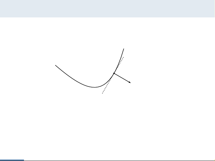
Basic inequality

Recall that for convex and differentiable f ,

(cid:73) The first-order approximation of f at x is a global lower

f (y ) f (x) + f (x)T (y x), x, y dom(f ). ≥ ∇ − ∀ ∈

(cid:73)

bound.

f defines a non-vertical supporting hyperplane to epi(f ) at

∇ (x, f (x)) (cid:33) (cid:32) (cid:33)(cid:33) (cid:16) f 0, (y , t) epi(f ). (cid:32)(cid:32) y t − ≤ ∀ ∈ ∇ (cid:17) 1 − x f (x)

g1 and g2 are subgradients at x1, g3 is subgradient at x2.

Subgradients

n such that

A subgradient of a convex function f at x is any g R

f (y ) f (x) + g T (y x), ∈ dom(f ). ≥ y ∀ ∈ −

(cid:73) Always exists (on the relative interior of dom(f )) (cid:73) If f differentiable at x, then g = f (x) uniquely (cid:73) Same definition works for nonconvex f (however, subgradients

∇

need not exist).

Subgradients

n such that

A subgradient of a convex function f at x is any g R

f (y ) f (x) + g T (y x), ∈ dom(f ). ≥ y ∀ ∈ −

(cid:73) Always exists (on the relative interior of dom(f )) (cid:73) If f differentiable at x, then g = f (x) uniquely (cid:73) Same definition works for nonconvex f (however, subgradients

∇

need not exist).

g1 and g2 are subgradients at x1, g3 is subgradient at x2.

Examples of subgradients

x Consider f : R R, f (x) = → | |

(cid:73) For x (cid:73) For x = 0, subgradient g is any element of [

= 0, unique subgradient g = sign(x) (cid:54) 1, 1]. −

Examples of subgradients

(cid:73) For x

Consider f : R R, f (x) = x (cid:107) (cid:107)2 →

(cid:73) For x = 0, subgradient g is any element of

= 0, unique subgradient g = x x (cid:54) (cid:107) (cid:107)2 z . z : { (cid:107) (cid:107)2 ≤ 1 }

Examples of subgradients

Consider f : R R, f (x) = x (cid:107) (cid:107)1 →

(cid:73) For xi = 0, unique ith component gi = sign(xi ) (cid:73) For xi = 0, ith component gi is any element of [

(cid:54) 1, 1]. −

Examples of subgradients

, for f1, f2 : R R convex, f1(x), f2(x) } → Consider f (x) = max { differentiable

(cid:73) For f1(x) > f2(x), unique subgradient g = (cid:73) For f2(x) > f1(x), unique subgradient g = (cid:73) For f1(x) = f2(x), subgradient g is any point on line segment

f1(x) f2(x) ∇ ∇

between f1(x) and f2(x). ∇ ∇

(cid:73) Nonempty for convex f at x

Properties:

(cid:73) ∂f (x) is closed and convex (even for nonconvex f )

(cid:73) If f is differentiable at x, then ∂f (x) =

int(domf ) ∈

(cid:73) If ∂f (x) =

f (x) } {∇ g , then f is differentiable at x and f (x) = g . { } ∇

Proof: See http://www.seas.ucla.edu/~vandenbe/236C/

lectures/subgradients.pdf

Subdifferential

Set of all subgradients of convex f is called the subdifferential:

n : g is a subgradient of f at x

g ∂f (x) = . R { ∈ }

Subdifferential

Set of all subgradients of convex f is called the subdifferential:

n : g is a subgradient of f at x

g ∂f (x) = . R { ∈ }

(cid:73) Nonempty for convex f at x

Properties:

(cid:73) ∂f (x) is closed and convex (even for nonconvex f )

(cid:73) If f is differentiable at x, then ∂f (x) =

int(domf ) ∈

(cid:73) If ∂f (x) =

{∇ f (x) } , then f is differentiable at x and f (x) = g . g { } ∇

Proof: See http://www.seas.ucla.edu/~vandenbe/236C/ lectures/subgradients.pdf

Question: Monotonicity for differentiable convex function?

f (x) ( f (y ))T (x y ) 0, ∇ − ∇ ≥ − which follows directly from the first order characterization of

convex functions.

Monotonicity

Theorem The subdifferential of a convex function f is a monotone operator

u v )T (x (u y ) 0, ∂f (x), v ∂f (y ). − ∀ ∈ ≥ − ∈

Chứng minh.

By definition we have

f (y ) f (x) + uT (y x) and f (x) f (y ) + v T (x y ). ≥ − ≥ − Combining them get shows monotonicity.

f (x) ( f (y ))T (x y ) 0, ∇ − ∇ ≥ − which follows directly from the first order characterization of

convex functions.

Monotonicity

Theorem The subdifferential of a convex function f is a monotone operator

u v )T (x (u y ) 0, ∂f (x), v ∂f (y ). − ∀ ∈ ≥ − ∈

Chứng minh.

By definition we have

f (y ) f (x) + uT (y x) and f (x) f (y ) + v T (x y ). ≥ − ≥ − Combining them get shows monotonicity.

Question: Monotonicity for differentiable convex function?

Monotonicity

Theorem The subdifferential of a convex function f is a monotone operator

u v )T (x (u y ) 0, ∂f (x), v ∂f (y ). − ∀ ∈ ≥ − ∈

Chứng minh.

By definition we have

f (y ) f (x) + uT (y x) and f (x) f (y ) + v T (x y ). ≥ − ≥ − Combining them get shows monotonicity.

Question: Monotonicity for differentiable convex function?

y ) 0, f (x) ( f (y ))T (x ≥ − ∇ − ∇

which follows directly from the first order characterization of convex functions.

Examples of non-subdifferentiable functions

(cid:73) f : R

The following functions are not subdifferentiable at x = 0

(cid:73) f : R

R, dom(f ) = R+ → (cid:40) f (x) = 1 if x = 0 0 if x > 0.

R, dom(f ) = R+ → √x. f (x) = −

The only supporting hyperplane to epi(f ) at (0, f (0)) is vertical.

Connection to convex geometry

n, consider indicator function IC : R  0 

C (x), the normal cone of C at x is, recall g T y for any y

n : g T x

C =

Convex set C R R, ⊆ → if x C x C ∈ = IC (x) = I { ∈ } if x C .  (cid:54)∈ ∞ For x C , ∂IC (x) = ∈ N C . R ∈ } N ≥ ∈

(cid:73) For y

x) for all y . g { Why? By definition of subgradient g , IC (x) + g T (y IC (y ) ≥ −

(cid:73) For y

C , IC (y ) = ∞ (cid:54)∈ C , this means 0 g T (y x). ∈ − ≥

Subgradient calculus

(cid:73) Scaling: ∂(af ) = a

Basic rules for convex functions:

(cid:73) Addition: ∂(f1 + f2) = ∂f1 + ∂f2. (cid:73) Affine composition: if g (x) = f (Ax + b), then

∂f provided a > 0. ·

(cid:73) Finite pointwise maximum: if f (x) = maxi=1,...m fi (x), then

∂g (x) = AT ∂f (Ax + b).

i:fi (x)=f (x)

(cid:19) (cid:18) (cid:91) ∂f (x) = conv ∂fi (x)

convex hull of union of subdifferentials of active functions at x.

Subgradient calculus

(cid:73) General pointwise maximum: if f (x) = maxs∈S fs (x), then

s:fs (x)=f (x)

(cid:19)     (cid:18) (cid:91) ∂f (x) cl conv . ∂fs (x) ⊇  

(cid:73) Norms: important special case, f (x) =

x Under some regularity conditions (on S, fs ), we get equality. (cid:107)p. Let q be such (cid:107) that 1/p + 1/q = 1, then

z T x. x (cid:107) (cid:107)p = max (cid:107)z(cid:107)q≤1

And

∂f (x) = argmax(cid:107)z(cid:107)q≤1 z T x.

Why subgradients?

(cid:73) Convex analysis: optimality characterization via subgradients,

Subgradients are important for two reasons:

(cid:73) Convex optimization: if you can compute subgradients, then

monotonicity, relationship to duality.

you can minimize any convex function.

Why? Easy: g = 0 being a subgradient means that for all y

f (y ) f (x ∗) + 0T (y x ∗) = f (x ∗). ≥ − Note the implication for a convex and differentiable function f

. with ∂f (x) = f (x) } {∇

Optimality condition

Subgradient optimality condition: For any f (convex or not),

0 f (x ∗) = min ∂f (x ∗), ⇐⇒ ∈ f (x) i.e., x ∗ is a minimizer if and only if 0 is a subgradient of f at x ∗.

Optimality condition

Subgradient optimality condition: For any f (convex or not),

0 f (x ∗) = min ∂f (x ∗), ⇐⇒ ∈ f (x) i.e., x ∗ is a minimizer if and only if 0 is a subgradient of f at x ∗.

Why? Easy: g = 0 being a subgradient means that for all y f (x ∗) + 0T (y x ∗) = f (x ∗). f (y ) ≥ −

. Note the implication for a convex and differentiable function f with ∂f (x) = f (x) } {∇

Derivation of first-order optimality

Example of the power of subgradients: we can use what we have learned so far to derive the first-order optimality condition.

Theorem For f convex and differentiable and C convex

C f (x) subject to x min x ∈

0 for all y is solved at x if and only if f (x)T (y x) C .a ∇ − ∈

≥ aDirect proof see, e.g., http://www.princeton.edu/~amirali/Public/ Teaching/ORF523/S16/ORF523_S16_Lec7_gh.pdf. Proof using subgradient next slide.

n (unconstrained case) it reduces to

Intuitively: says that gradient increases as we move away from x.

f = 0. Note that for C = R ∇

Derivation of first-order optimality

Chứng minh.

First recast problem as

f (x) + IC (x). min x

∂(f (x) + IC (x)). ∈ Now apply subgradient optimality: 0 Observe

C (x)

0 0 + ∂(f (x) + IC (x)) ∈ f (x) } ⇔ N C (x) ∈ N ⇔ −∇ C f (x)T y for all y ⇔ −∇ ∈ 0 for all y C ∈ {∇ f (x) f (x)T x f (x)T (y ≥ −∇ x) ⇔ ∇ ≥ − ∈ as desired.

∂f (x) + ∈

Note: the condition 0 C (x) is a fully general condition N for optimality in convex problems. But it’s not always easy to work with (KKT conditions, later, are easier).

2 + λ

Subgradient optimality (cid:19) (cid:18) 1 0 y 0 ∂ X β β X T (y X β) + λ∂ β ∈ 2 (cid:107) − (cid:107) (cid:107) (cid:107)1 ⇔ ∈ − − (cid:107) (cid:107)1

X T (y X β) = λv ⇔ − for some v ∂ β (cid:107)1, i.e., (cid:107) ∈  1 if βi > 0 { }  1 vi i = 1, . . . , p. if βi < 0, ∈ {− }  [ 1, 1] if βi = 0 −

Example: lasso optimality conditions

n×p, lasso problem can be parametrized as

n, X

2 2 + λ

Given y R R ∈ ∈ X β β min β 1 y 2 (cid:107) − (cid:107) (cid:107) (cid:107)1 0. where λ ≥

Example: lasso optimality conditions

n×p, lasso problem can be parametrized as

n, X

2 2 + λ

2 2 + λ (cid:107)

Given y R R ∈ ∈ X β β min β 1 y 2 (cid:107) − (cid:107) (cid:107)1 (cid:107) 0. Subgradient optimality where λ (cid:19) ≥ (cid:18) 1 0 0 ∂ X β β X T (y X β) + λ∂ ∈ y 2 (cid:107) − (cid:107) (cid:107)1 − β (cid:107) (cid:107)1 ⇔

∈ − X T (y X β) = λv ⇔ − for some v ∂ β (cid:107) ∈ if βi > 0

vi i = 1, . . . , p. if βi < 0, ∈ if βi = 0 (cid:107)1, i.e.,  1  } { 1 } {−  1, 1] [ −

Note: subgradient optimality conditions don’t lead to closed-form

expression for a lasso solution. However they do provide a way to

check lasso optimality.

They are also helpful in understanding the lasso estimator; e.g., if

i (y

X T X β) < λ, then βi = 0 (used by screening rules, later?). | − |

Example: lasso optimality conditions

Write X1, . . . , Xp for columns of X . Then our condition reads

  X β) = λ = 0 sign(βi ) if βi − (cid:54) · λ X β) if βi = 0. X T i (y X T i (y  | − | ≤

Example: lasso optimality conditions

Write X1, . . . , Xp for columns of X . Then our condition reads

  X β) = λ = 0 sign(βi ) if βi − (cid:54) · λ X β) if βi = 0. X T i (y X T i (y  | − | ≤

Note: subgradient optimality conditions don’t lead to closed-form expression for a lasso solution. However they do provide a way to check lasso optimality.

i (y

They are also helpful in understanding the lasso estimator; e.g., if X T < λ, then βi = 0 (used by screening rules, later?). X β) | − |

Example: soft-thresholding

Simplfied lasso problem with X = I :

2 2 + λ

y β β min β 1 2 (cid:107) − (cid:107)1 . (cid:107)

(cid:107) This we can solve directly using subgradient optimality. Solution is β = Sλ(y ), where Sλ is the soft-thresholding operator

λ if yi > λ − if λ, i = 1, . . . , n. λ [Sλ(y )]i = yi − ≤ ≤  yi  0  λ yi + λ if yi < − Check: from last slide, subgradient optimality conditions are

  = 0 yi βi = λ sign(βi ) if βi − (cid:54) · λ yi βi if βi = 0.  | − | ≤

Example: soft-thresholding

Now plug in β = Sλ(y ) and check these are satisfied:

(cid:73) When yi > λ, βi = yi (cid:73) When yi < (cid:73) When

1. βi = λ = λ − − ·

= λ. λ > 0, so yi λ, argument is similar. λ, βi = 0, and βi yi − | ≤ yi | yi | − | | | ≤

Soft-thresholding in one variable

x Write dist(x, C ) = PC (x) (cid:107) − (cid:107)2, where PC (x) is the projection of x onto C . It turns out that when dist(x, C ) > 0, (cid:27) (cid:26) x PC (x) ∂ dist(x, C ) = − x PC (x) − (cid:107) (cid:107)2 only has one element, so in fact dist(x, C ) is differentiable and this is its gradient.

Example: distance to a convex set

Recall the distance function to a closed, convex set C

y ∈C (cid:107)

y x dist(x, C ) = min − (cid:107)2 . This is a convex function. What are its subgradients?

Example: distance to a convex set

Recall the distance function to a closed, convex set C

y ∈C (cid:107)

y x dist(x, C ) = min − (cid:107)2 . This is a convex function. What are its subgradients?

PC (x) x (cid:107) Write dist(x, C ) = − x onto C . It turns out that when dist(x, C ) > 0,

∂ dist(x, C ) = PC (x) PC (x) − − (cid:107)2

(cid:107)2, where PC (x) is the projection of (cid:27) (cid:26) x x (cid:107) only has one element, so in fact dist(x, C ) is differentiable and this is its gradient.

Example: distance to a convex set

∂ dist(x, C ). PC (x) PC (x) We will only show one direction, i.e., that x x (cid:107) − −

(cid:107)2 ∈ Write u = PC (x). Then by first-order optimality conditions for a projection,

0 for all y u)T (y (x u) C . − − ≤ ∈ Hence

C H = y : (x u)T (y u) . ⊆ { − 0 } ≤ − Claim (x u) dist(y , C ) for all y . u)T (y u x ≥ − (cid:107)2 − (cid:107) − H, the right-hand side is 0. Check: first, for y ≤ ∈

Example: distance to a convex set

x u − (cid:107)2 cos θ where θ is the angle − y u (cid:107)2 (cid:107) u. Thus

H, we have u) = (cid:107) u and y u) y u − − = dist(y , C ) (cid:107) (cid:107)2 cos θ = dist(y , H) − ≤ − (cid:107) − − (cid:107)2 Now for y (cid:54)∈ u)T (y (x − between x − u)T (y (x u x as desired.

(x u) dist(y , C ) − − Using the claim, we have for any y u)T (y x ≥ (cid:19)T x u = (y x) u u − x + x − u (cid:107)2 − (cid:107) (cid:18) x (cid:107)2 + x (cid:107) − − Hence g = (x u)/ − (cid:107) x (cid:107) − − (cid:107)2 (cid:107)2 is a subgradient of dist(x, C ) at x. u

References and further reading

S. Boyd, Lecture notes for EE 264B, Stanford University, Spring 2010-2011

R. T. Rockafellar (1970), Convex analysis, Chapters 23–25

L. Vandenberghe, Lecture notes for EE 236C, UCLA, Spring 2011-2012

Bài giảng Tối ưu hóa nâng cao: Chương 6 - Hoàng Nam Dũng