Genet. Sel. Evol. 39 (2007) 669–683 Available online at:
c
INRA, EDP Sciences, 2007 www.gse-journal.org
DOI: 10.1051/gse:2007031 Original article
Analysis of a simulated microarray dataset:
Comparison of methods for
data normalisation and detection
of differential expression
(Open Access publication)
Michael W a∗, Mónica P´
-Ab, Michael Denis
Bc, Céline Dd, Peter D ˇ
e,MylèneDd,
Jean-Louis Ff, Juan José G-P ´
b,Ina
Hg,FlorenceJ´
f, Ángeles J´
-M´
b,
Miha L ˇ
e,Kim-AnhL
ˆ
Ch, Guillemette Mf, Daphné
Mh, Marco H. Pc, Christèle R-G´
d, Magali
S Cd, Gwenola T-Kd,David
Wh,Dirk-Jan Kh
aInstitute for Animal Health, Compton, UK (IAH_C)
bUniversity of Cordoba, Cordoba, Spain (CDB)
cInstitute for Animal Health, Pirbright, UK (IAH_P)
dINRA, Castanet-Tolosan, France (INRA_T)
eUniversity of Ljubljana, Slovenia (SLN)
fINRA, Jouy-en-Josas, France (INRA_J)
gAnimal Sciences Group Wageningen UR, Lelystad, NL (IDL)
hRoslin Institute, Roslin, UK (ROSLIN)
(Received 10 May 2007; accepted 10 July 2007)
Abstract – Microarrays allow researchers to measure the expression of thousands of genes in
a single experiment. Before statistical comparisons can be made, the data must be assessed
for quality and normalisation procedures must be applied, of which many have been proposed.
Methods of comparing the normalised data are also abundant, and no clear consensus has yet
been reached. The purpose of this paper was to compare those methods used by the EADGENE
network on a very noisy simulated data set. With the aprioriknowledge of which genes are
differentially expressed, it is possible to compare the success of each approach quantitatively.
Use of an intensity-dependent normalisation procedure was common, as was correction for
∗Corresponding author: michael.watson@bbsrc.ac.uk
Institute for Animal Health Informatic groups, Compton Laboratory, Compton RG20 7 NN
Newbury Bershive, UK.
Article published by EDP Sciences and available at http://www.gse-journal.org
or http://dx.doi.org/10.1051/gse:2007031

670 M. Watson et al.
multiple testing. Most variety in performance resulted from differing approaches to data quality
and the use of different statistical tests. Very few of the methods used any kind of background
correction. A number of approaches achieved a success rate of 95% or above, with relatively
small numbers of false positives and negatives. Applying stringent spot selection criteria and
elimination of data did not improve the false positive rate and greatly increased the false negative
rate. However, most approaches performed well, and it is encouraging that widely available
techniques can achieve such good results on a very noisy data set.
gene expression /two colour microarray /simulation /statistical analysis
1. INTRODUCTION
Microarrays have become a standard tool for the exploration of global gene
expression changes at the cellular level, allowing researchers to measure the
expression of thousands of genes in a single experiment [16]. The hypothesis
underlying the approach is that the measured intensity for each gene on the ar-
ray is proportional to its relative expression. Thus, biologically relevant differ-
ences, changes and patterns may be elucidated by applying statistical methods
to compare different biological states for each gene. However, before com-
parisons can be made, a number of normalisation steps should be taken in
order to remove systematic errors and ensure the gene expression measure-
ments are comparable across arrays [15]. There is no clear consensus in the
community about which methods to use, though several reviews have been
published [8, 12]. After normalisation and statistical tests have been applied,
there is an additional problem of multiple testing. Due to the high number of
tests taking place (many thousands in most cases), the resulting P-values must
be adjusted in order to control or estimate the error rate (see [14] for a review).
The aim of this paper was to summarise and compare the many methods
used throughout the EADGENE network (http://www.eadgene.org) for mi-
croarray analysis, and compare the results, with the final aim of producing
a guide for best practice within the network [4]. This paper describes a variety
of methods applied to a simulated data set produced by the SIMAGE pack-
age [1]. The data set is a simple comparison of two biological states on ten
arrays, with dye-balance. A number of data quality, normalisation and analysis
steps were used in various combinations, with differing results.
1.1. The data
SIMAGE takes a number of parameters, which were produced using a slide
from the real data set as an example [4]. The input values that were used for
the current simulations are given in Table I. The simulated data consists of

Data normalisation of gene expression analysis 671
ten microarrays each of which represent a direct comparison between differ-
ent biological samples from situation A and B with a dye balance. SIMAGE
assumes a common variance for all genes, something which may not be true
for real data. Each slide had 2400 genes in duplicate, with 48 blocks arranged
in 12 rows and 4 columns (100 spots per block). Each block was “printed”
with a unique print tip. In the simulated data 624 genes were differentially
expressed: 264 were up-regulated from A to B while 360 were down regu-
lated. This information was only provided to the participants at the end of the
workshop. The simulated data are available upon request from D.J. de Koning
(DJ.dekoning@bbsrc.ac.uk).
The data are very noisy with high levels of technical bias and thus provided
a serious challenge for the various analysis methods that were applied. Many
spots reported background higher than foreground, and others reported a zero
foreground signal. Image plots of the arrays showed clear spatial biases in both
foreground and background intensities (Fig. 1). Spots, scratches and stripes of
background variation are clearly visible, which have been simulated using the
“hair” and “disc” parameters of SIMAGE.
All of the slides show a clear relationship between M (log ratio) and A
(average log intensity), and the plots in Figure 2 are exemplars. Slides 3, 5,
6, 7, 9 and 10 displayed a negative relationship between M and A, whilst the
others displayed a positive relationship. Slides 6 and 9 showed an obvious non-
linear relationship between M and A, but only slide 2 levels offwith higher
values of A. Finally, Figure 3 shows the range of M values for each array
under three different normalisation strategies: none (Fig. 3a), LOESS (Fig. 3b)
and LOESS followed by scale normalisation between arrays (Fig. 3c) [17,19].
It can be seen that before normalisation there is a clear difference in both the
median log ratios and the range of log ratios across slides.
This data set was subject to a total of 12 different analysis methods, encom-
passing a variety of techniques for assessing data quality, normalisation and
detecting differential expression. These methods are described in detail and
the results of each presented and compared. The results are then discussed in
relation to the best methods to use for analysing extremely noisy microarray
data.
2. MATERIALS AND METHODS
2.1. Preprocessing and normalisation procedures
A variety of pre-processing and normalisation procedures were used in
combination with the twelve different methods, and these are summarised in

672 M. Watson et al.
Tab le I. Settings for Simage simulation software.
Array number of grid rows 12
Array number of grid columns 4
Number of spots in a grid row 10
Number of spots in a grid column 10
Number of spot pins 48
Number of technical replicates 2
Number of genes 0
Number of slides 10
Perform dye swaps yes
Gene expression filter yes
Reset gene filter for each slide no
Mean signal 10.33
Change in log2ratio due to upregulation 1.07
Change in log2ratio due to downregulation –1.26
Variance of gene expression 2.7
% of upregulated genes 15
% of downregulated genes 11
Correlation between channels 1
Dye filter yes
Reset dye filter for each slide yes
Channel variation 0.2
Gene ×Dye 0
Error filter yes
Reset error filter for each slide yes
Random noise standard deviation 0.62
Tail behaviour in the MA plot 0.108
Non-linearity filter yes
Reset non-linearity filter for each slide yes
Non-linearity parameter curvature 0.2
Non-linearity parameter tilt 4.5
Non-linearity from scanner filter yes
Reset non-linearity scanner filter for each slide yes
Scanning device bias 0.04
Spotpin deviation filter yes
Reset spotpin filter for each slide no
Spotpin variation 0.32
Background filter yes
Reset background filter for each slide yes
Number of background densities 5
Mean standard deviation per background density 0.2
Maximum of the background signal relative to the non-background signals 50
Standard deviation of the random noise for the background signals 0.1
Background gradient filter no
Reset gradient filter for each slide yes
Maximum slope of the linear tilt 700
Missing values filter yes
Reset missing spots filter for each slide yes
Number of hairs 3
Maximum length of hair 20
Number of discs 4
Average radius disc 10
Number of missing spots 50

Data normalisation of gene expression analysis 673
Figure 1. Example background plots. The top two images show the background for
Cy5 and Cy3 in slide 9, and the bottom two images show the same for slide 10.
Table II. Only one method, IDL1, chose to perform background correction.
Some methods chose to eliminate spots, or give them zero weighting, depend-
ing on particular data quality statistics; these included having foreground less
than a given multiple of background, saturated spots and spots whose inten-
sity was zero. IAH_P1 and IDL1 also removed entire slides considered to have
poor data quality. Both IAH_P and IDL submitted two approaches, one based
on strict quality control and normalisation, and the second less strict.
Most approaches applied a version of LOWESS or LOESS normalisation,
either globally or per print-tip [19]. This is in recognition of the clear rela-
tionship between M and A. Only ROSLIN (assessed normalisation by row and