Nguyễn Công Phương
CONTROL SYSTEM DESIGN
State Variable Models
Contents
Introduction
I. II. Mathematical Models of Systems III. State Variable Models IV. Feedback Control System Characteristics V. The Performance of Feedback Control Systems VI. The Stability of Linear Feedback Systems VII. The Root Locus Method VIII.Frequency Response Methods IX. Stability in the Frequency Domain X. The Design of Feedback Control Systems XI. The Design of State Variable Feedback Systems XII. Robust Control Systems XIII.Digital Control Systems
sites.google.com/site/ncpdhbkhn
2
State Variable Models
1. The State Variables of a Dynamic System 2. The State Differential Equation 3. Signal – Flow Graph & Block Diagram Models 4. Alternative Signal – Flow Graph & Block
Diagram Models
5. The Transfer Function from the State Equation 6. The Time Response & the State Transition
Matrix
7. Analysis of State Variable Models Using Control
Design Software
sites.google.com/site/ncpdhbkhn
3
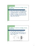
The State Variables of a Dynamic System (1)
• The state of a system is a set of variables
whose values, together with the input signals & the equations describing the dynamics, will provide the future state & output of the system.
• The state variables describe the present
configuration of a system & can be used to determine the future response, given the excitation inputs & the equations describing the dynamics.
sites.google.com/site/ncpdhbkhn
4
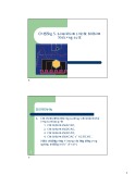
The State Variables of a Dynamic System (2)
Wall friction b
M b ky t ( ) u t ( )
2 d y t ( ) 2 dt
k
y t ( ),
x t ( ) 1
x t ( ) 2
dy t ( ) dt
Mass M
dy t ( ) dt
2
y(t)
u(t)
M
bx
u t ( )
2
kx 1
dx 2 dt
x
2
C
u t ( )
i
x u x 1 k M 1 M b M dx 1 dt dx 2 dt
i c
L
2
dv C dt
x u t ( )
L
Li C
R
1 C 1 C
L
Ri
2
v C
L
Cv
( )u t
Ci
t ( )
di L dt
x x 1 1 L R L dx 1 dt dx 2 dt ov
x
i
2
v o x 1
Ri L v ,C
2
L
sites.google.com/site/ncpdhbkhn
5
Rx v t ( ) o
State Variable Models
1. The State Variables of a Dynamic System 2. The State Differential Equation 3. Signal – Flow Graph & Block Diagram Models 4. Alternative Signal – Flow Graph & Block
Diagram Models
5. The Transfer Function from the State Equation 6. The Time Response & the State Transition
Matrix
7. Analysis of State Variable Models Using Control
Design Software
sites.google.com/site/ncpdhbkhn
6
The State Differential Equation (1) ...
...
...
...
x 1 x
a x 11 1 a x 21 1
a x 12 2 a x 22 2
a x 1 n n a x 2 n n
b u 11 1 b u 21 1
b u 1 m m b u 2 m m
2
...
...
n
a x 1 1 n
a x 2 2 n
a x nn n
b u 1 1 n
b u nm m
x
x 1 x
a 11 a
a 1 n a
a 12 a
x 1 x
n
d dt
b b 11 1 m b b nm n 1
u 2 u m
2 x
21 a
2 x
22 2 a a
n
n 1
nn
n
2
n
x Ax Bu y Cx Du
t
t
x
t ( )
exp(
A x t
) (0)
exp[
A
(
t
)
Bu
t
)
r d ( )
( )
d
t ( ) (0) Φ x
( Φ
Bu
0
0
1
1
X
[
s
I A x ]
(0)[
I A BU s ]
s ( )
s ( )
sites.google.com/site/ncpdhbkhn
7
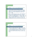
The State Differential Equation (2)
x
u t ( )
2
1 C
1 C
x
x 1
2
1 L
R L
dx 1 dt dx 2 dt
L
Li C
R
Rx
Cv
v t ( ) o
2
( )u t
Ci
ov
0
x u t ( ) x
1 C 0
sites.google.com/site/ncpdhbkhn
8
1 C R L x R 1 L 0 y
The State Differential Equation (3)
q
p
1k
2k
u
f
f
u
M a 1 1
spring
damp
M2
M1
)
(
)
M p 1
u k p q ( 1
b p q 1
1b
2b
M p b p k p 1
1
1
u k q b q 1 1
(
)
(
)
M q 2
k p q 1
b p q 1
k q b q 2
2
(
(
M q 2
k 1
k q ) 2
b 1
b q ) 2
k p b p 1
1
p
,
q
x 3 x
x 1 x
p q
2
4
2
x 1 x
b 1 M
1
1
1
p u q p p q x 3 k 1 M 1 M k 1 M b 1 M
2
4
1 b 1 M
2
2
2
2
1 k 1 M sites.google.com/site/ncpdhbkhn
9
k b 2 q p q p x q k 1 M b 1 M
The State Differential Equation (4)
1
1
1
p u q p p q x 3 k 1 M b 1 M 1 M k 1 M b 1 M
2
4
1 k 1 M
1 b 1 M
2
2
2
2
k b 2 q p q p x q k 1 M b 1 M
p
,
2
4
2
x
u
x
x 3
x 1
2
x 3
4
k 1 M
k 1 M
b 1 M
b 1 M
1 M
1
1
b 2
2
x
x
x
4
4
x 1
2
x 3
k 1 M
1 k k 1 M
1 b 1 M
1 b 1 M
2
2
2
2
sites.google.com/site/ncpdhbkhn
10
q x 3 x x 1 x p q x 1 x
4
2
The State Differential Equation (5) b 1 M
1
1
u x x x 3 x 3 x 1 k 1 M k 1 M b 1 M 1 M
2
4
4
2
1 k k 1 M
1 b 1 M
1 b 1 M
2
2
2
2
0
0
b 2 x x x x 1 x 3 k 1 M
A
,
B
x
,
0 0 k 1 M
0 0 k 1 M
1 0 b 1 M
0 1 b 1 M
1
1
1 M
1
k
x 1 x 2 x 3 x
2
b 2
4
p q p q
0
k 1 M
1 k 1 M
b 1 M
1 b 1 M
2
2
2
2
x Ax B u
y
p
x Cx
1 0 0 0
x 1
sites.google.com/site/ncpdhbkhn
11
The State Differential Equation (6)
q
p
1k
2k
u
M2
M1
1b
2b
x
u
x
x 3
x 1
2
x 3
4
k 1 M
k 1 M
b 1 M
b 1 M
1 M
1
1
b 2
2
x
x
x
4
4
x 1
2
x 3
k 1 M
1 k k 1 M
1 b 1 M
1 b 1 M
2
2
2
2
p
q
)
)
p
u
M2
M2
)
)
p
k p q 1( b p q 1(
2k q 2b q
k q 1( b q 1(
sites.google.com/site/ncpdhbkhn
12
State Variable Models
1. The State Variables of a Dynamic System 2. The State Differential Equation 3. Signal – Flow Graph & Block Diagram
Models
4. Alternative Signal – Flow Graph & Block
Diagram Models
5. The Transfer Function from the State Equation 6. The Time Response & the State Transition
Matrix
7. Analysis of State Variable Models Using Control
Design Software
sites.google.com/site/ncpdhbkhn
13
Signal – Flow Graph & Block Diagram Models (1)
L
x
u t ( )
2
1 C
1 C
Li C
R
ov
( )u t
Ci
x
x 1
2
1 L
R L
dx 1 dt dx 2 dt
R L
1 L
1 s
R
1 C
Rx
v t ( ) o
2
( )U s
Cv
?
oV s ( )
1/ s
1X
2X
2
1 C
oV s ( ) U s ( )
G s ( )
( )
( )U s
1X
oV s ( )
R
1 L
R L 2X1 s
1 s
1 C
( )
1 C
sites.google.com/site/ncpdhbkhn
14
LC ) s ( ) /( R LC R L s ) / 1/(
Signal – Flow Graph & Block Diagram Models (2)
m
m
1
b m
G s ( )
,
n m
( ) Y s U s ( )
b s m n s
a
s 1 1 n s
... ...
n
b s b 1 0 a s a 1
0
1
n m
)
(
1)
1)
n
(
n m
( n
b s m
b m
b s 0
n
s 1 1 s
s a
...
b s 1 1)
n
... ( n a s 1
a s 0
1
P k
k
N
Sum of the forward-path factor 1 sum of the feedback loop factors
1
L q
q
1
sites.google.com/site/ncpdhbkhn
15
Signal – Flow Graph & Block Diagram Models (3)
Ex. 1
4
G s ( )
4
3
1
3
4
2
b s 0 2
Y s ( ) U s ( )
s
1
a s 3
a s a 1
0
a s 3
a s 2
a s 1
a s 0
b 0 a s 2
4
3
2
)
a s 2
s ( 4
3
d
)
d
d
)
)
(
)
a
a
/
)
u
3
2
a y b ( 0
0
a 1
d y b / 0 dt
a s a Y s ( ) 1 0 2 y b / ( 0 3 dt
b U s ( ) 0 y b / ( 0 2 dt
4X
1
1 s
1 s
1 s
1 s
0b
( )U s
( )Y s
x 1 x
a s 3 y b / ( 0 4 dt y b / 0
3X
2X
1X
2
3a
2a
1a
x 3 x
0a
4
x 1 x 2 x 3
y b / 0 y b / 0 y b / 0
4X
3X
2X
1X
( )Y s
( )U s
0b
1 s
1 s
1 s
1 s
1 s
( )
( )
3a
2a
( )
1a
0a
( ) sites.google.com/site/ncpdhbkhn
16
Signal – Flow Graph & Block Diagram Models (4)
Ex. 1
4
G s ( )
4
3
1
3
4
2
b s 0 2
Y s ( ) U s ( )
s
1
a s 3
a s a 1
0
a s 3
a s 2
a s 1
a s 0
b 0 a s 2
4
3
2
d
)
d
)
d
)
)
(
a
a
/
)
u
3
2
a 1
a y b ( 0
0
/ d y b 0 dt
( y b / 0 4 dt
( y b / 0 3 dt
( y b / 0 2 dt
x 1 x
y b / 0
2
x 3 x
4
x 1 x 2 x 3
y b / 0 y b / 0 y b / 0
u
x 4
a x 0 1
a x 1 2
a x 2 3
a x 3 4
y
b x 0 1
sites.google.com/site/ncpdhbkhn
17
Signal – Flow Graph & Block Diagram Models (5)
Ex. 1
4
G s ( )
4
3
1
3
4
2
b s 0 2
Y s ( ) U s ( )
s
1
a s 3
a s a 1
0
a s 3
a s 2
a s 1
a s 0
b 0 a s 2
u
x
4
a x 0 1
a x 1 2
a x 2 3
a x 3 4
y
b x 0 1
u t ( )
x Ax B u
0 0 0 a
0 0 0 a
0 0 0 a
x 1 x 2 x 3 x
x 1 x 2 x 3 x
0 0 0 a 1
0
2
3
4
4
0 0 0 1
x 1 x
y t ( )
Cx
0 0 0
b 0
2 x 3
x 4 sites.google.com/site/ncpdhbkhn
18
Signal – Flow Graph & Block Diagram Models (6)
Ex. 1
4
G s ( )
4
3
1
3
4
2
b s 0 2
Y s ( ) U s ( )
s
1
a s 3
a s a 1
0
a s 3
a s 2
a s 1
a s 0
b 0 a s 2
4X
1
1 s
1 s
1 s
1 s
0b
( )U s
( )Y s
3X
2X
1X
3a
2a
1a
0a
P k
k
G s ( )
N
Y s ( ) U s ( )
Sum of the forward-path factor 1 sum of the feedback loop factors
1
L q
q
1
4X
3X
2X
1X
( )Y s
( )U s
0b
1 s
1 s
1 s
1 s
( )
( )
3a
2a
( )
1a
0a
( ) sites.google.com/site/ncpdhbkhn
19
Ex. 2
2
1
3
2
3
4
G s ( )
1
4
4
2
Y s ( ) U s ( )
1
s
b s 2
b s 3
Signal – Flow Graph & Block Diagram Models (7) b s 0 3 a s 0
b s b 1 0 a s a 1
b s 2 a s 2
b s 3 a s 3
b s 1 a s 1
2 a s 2
0
P k
k
G s ( )
N
( ) Y s U s ( )
Sum of the forward-path factor 1 sum of the feedback loop factors
1
L q
3 a s 3
q
1
3b
2b
4X
1b
1
1 s
1/ s
1/ s
1/ s
0b
( )U s
( )Y s
3X
2X
1X
3a
2a
1a
0a
sites.google.com/site/ncpdhbkhn
20
Ex. 2
1
2
3
3
4
2
G s ( )
1
4
4
2
Y s ( ) U s ( )
1
s
b s 2
b s 3
Signal – Flow Graph & Block Diagram Models (8) b s 0 3 a s 0
b s b 1 0 a s a 1
b s 2 a s 2
b s 3 a s 3
b s 1 a s 1
2 a s 2
3 a s 3
0
3b
2b
4X
1b
1
1 s
1/ s
1/ s
1/ s
0b
( )U s
( )Y s
3X
2X
1X
3a
2a
1a
0a
X
1
X
2
X
X s / 2 X s / 3 X s / 4
3
X
) /
s
U a X (
a X 0
1
2
Y
4
3
4 b X 0
1
3 b X 1
2
a X 2 b X 2
3
a X 1 b X 3
4
sites.google.com/site/ncpdhbkhn
21
Ex. 2
2
1
3
2
3
4
G s ( )
1
4
4
2
Y s ( ) U s ( )
1
s
b s 2
b s 3
Signal – Flow Graph & Block Diagram Models (9) b s 0 3 a s 0
b s b 1 0 a s a 1
b s 2 a s 2
b s 3 a s 3
b s 1 a s 1
2 a s 2
3 a s 3
0
X
X
sX
1
2
1
X
X
sX
2
3
2
X
X
sX
X s / 2 X s / 3 X s / 4
3
4
3
X
sX
) /
s
)
U a X (
U a X (
a X 0
1
2
a X 0
1
2
4
3
4
3
3 b X 1
2
a X 2 b X 2
3
a X 1 b X 3
4
1
4 b X 0
1
3 b X 1
2
a X 2 b X 2
3
a X 1 b X 3
4
4 Y b X 0
Y
0
1
0
0
0
0
0
1
x 1 x
x 1 x
u t ( )
x
2
0
0
1
0
d dt
2 x 3
2 x 3
a
a
a
x
x
0
a 1
3
4
4
0 0 0 1
x 3 x
4
a x 0 1
2 x 1 x
y t ( )
b 0
b 1
b 2
b 3
x 1 x 2 x 3 u a x 3 4 b x 1 2
b x 0 1
a x 2 3 b x 2 3
a x 1 2 b x 3 4
x 4 y
2 x 3
x
4
sites.google.com/site/ncpdhbkhn
22
Ex. 2
2
3
G s ( )
4
Signal – Flow Graph & Block Diagram Models (10) Y s ( ) U s ( )
s
b s 2
b s 3
b s b 1 0 a s a 1
2 a s 2
3 a s 3
0
3
2
G s ( )
.
4
Y s ( ) U s ( )
( ) Z s Z s ( )
s
b s 3
b s 2
3 a s 3
2 a s 2
b s b 0 1 a s a 1
0
y
3
2
b 3
b 2
b 1
b z 0
(
)
b s 3
b s 2
b s b Z s ( ) 1 0
4
3
2
(
s
)
a s 3
a s 2
a s a Z s ( ) 1 0
Y s ( ) U s ( )
a
a
3
2
a 1
a z 0
dz dt
3 d z 3 dt 4 d z 4 dt
2 d z 2 dt 3 d z 3 dt
dz dt 2 d z 2 dt
u
x
2
z
2
x 3 x
4
a x 0 1
x 3 x
z z z
4
x 1 x 2 x 3
x 1 x
x 1 x 2 x 3 u a x 3 4 b x 1 2
b x 0 1
a x 2 3 b x 2 3
a x 1 2 b x 3 4
x 4 y
sites.google.com/site/ncpdhbkhn
23
Ex. 2
3
2
3b
G s ( )
4
Signal – Flow Graph & Block Diagram Models (11) Y s ( ) U s ( )
s
b s 2
b s 3
b s b 1 0 a s a 1
2 a s 2
3 a s 3
0
2b
4X
1b
1
1 s
1/ s
1/ s
1/ s
0b
x
( )U s
2
( )Y s
3X
2X
1X
3a
2a
1a
x 3 x
4
0a
a x 0 1
phase variable canonical form
x 1 x 2 x 3 u a x 3 4 b x 1 2
b x 0 1
a x 2 3 b x 2 3
a x 1 2 b x 3 4
x 4 y
3b
2b
1b
4X
3X
2X
1X
( )Y s
( )U s
0b
1 s
1 s
1 s
1 s
( )
( )
3a
2a
( )
1a
( )
0a
sites.google.com/site/ncpdhbkhn
24
Ex. 2
3
2
3b
G s ( )
4
Signal – Flow Graph & Block Diagram Models (12) Y s ( ) U s ( )
s
b s 2
b s 3
b s b 1 0 a s a 1
2 a s 2
3 a s 3
0
2b
4X
1b
1
1 s
1/ s
1/ s
1/ s
0b
( )U s
( )Y s
1X
3X
2X
3a
2a
1a
0a
phase variable canonical form
3b
2b
1x
2X
1X
1
1/ s
1/ s
1/ s
1b
1
( )Y s
( )U s
1/ s
1
1
4X
3X
0b
4x
3x
2x
2a
1a
3a
0a
input feedforward canonical form
sites.google.com/site/ncpdhbkhn
25
Ex. 2
3
2
G s ( )
4
Signal – Flow Graph & Block Diagram Models (13) Y s ( ) U s ( )
s
b s 2
b s 3
b s b 1 0 a s a 1
2 a s 2
3 a s 3
0
x
3
2 x 3
2
x u t ( )
x
b u 3 b u 2 b u 1
0
a x 3 1 a x 2 1 a x 1 1 a x 0 1
4 b u 0
x d dt
x 1
x 1 x x 3 x 4 y
3b
2b
1x
2X
1X
1
1/ s
1/ s
1/ s
1b
1
( )Y s
( )U s
1/ s
1
1
4X
3X
0b
4x
3x
2x
2a
1a
3a
0a
y t ( ) x a a 2 a 1 a 1 0 0 0 1 0 0 0 1 0 0 0 1 0 0 0 b 3 b 2 b 1 b 0 0 ( ) u t
input feedforward canonical form
sites.google.com/site/ncpdhbkhn
26
Ex. 2
3
2
G s ( )
4
Signal – Flow Graph & Block Diagram Models (14) Y s ( ) U s ( )
s
b s 2
b s 3
b s b 1 0 a s a 1
2 a s 2
3 a s 3
0
3b
2b
1x
2X
1X
1/ s
1
1/ s
1/ s
1b
1
( )Y s
( )U s
1/ s
1
1
4X
3X
0b
4x
3x
2x
2a
1a
3a
0a
3b
2b
1b
4x
3x
2x
1x
4X
3X
2X
1X
( )U s
( )Y s
0b
1 s
1 s
1 s
1 s
( )
( )
( )
( )
3a
2a
1a
0a
sites.google.com/site/ncpdhbkhn
27
Ex. 3
( )U s
( )Y s
G s ( )
s 3( s s (
s s
2) 4)
Signal – Flow Graph & Block Diagram Models (15) Y s ( ) 1)( 3)( U s ( )
T s ( )
( )
2
G 1 G
3
3
s 2 s 6
3
1
X1
X2
s
6
s
s 3 1 10
9
6 s s 2 s 21
G
( )
H
2X
1X
1
G GH
sites.google.com/site/ncpdhbkhn
28
3 s 10 1 9 6 s 21 s 2
Ex. 3
( )U s
( )Y s
2
1
3
G s ( )
s 3( s s (
s s
2) 4)
Signal – Flow Graph & Block Diagram Models (15) 1)( 3)(
3
( )
3
9
1
1/ s
1/ s
1/ s
6
( )U s
( )Y s
1X
3X
2X
10
21
6
1
2
3
4
T s ( )
1
4
2
3
1
b s 3 a s 3
b s 2 a s 2
b s 1 a s 1
b s 0 a s 0
3b
2b
4X
1b
1
1 s
1/ s
1/ s
1/ s
0b
( )U s
( )Y s
3X
2X
1X
3a
2a
1a
sites.google.com/site/ncpdhbkhn
29
0a
T s ( ) 1 s 6 s s 3 1 10 9 6 s s 2 s 21
Ex. 3
( )U s
( )Y s
2
3
1
G s ( )
s 3( s s (
s s
2) 4)
Signal – Flow Graph & Block Diagram Models (16) 1)( 3)(
3
( )
3
9
1
1/ s
1/ s
1/ s
6
( )U s
( )Y s
1X
3X
2X
10
21
6
3
9
3X
2X
1X
( )Y s
( )U s
6
1 s
1 s
1 s
( )
10
21
( )
6
sites.google.com/site/ncpdhbkhn
30
T s ( ) 1 s 6 s s 3 1 10 9 6 s s 2 s 21
Ex. 3
( )U s
( )Y s
1
2
3
G s ( )
s 3( s s (
s s
2) 4)
Signal – Flow Graph & Block Diagram Models (17) 1)( 3)(
3
( )
3
9
1
1/ s
1/ s
1/ s
6
( )U s
( )Y s
1X
3X
2X
10
21
6
0
1
0
x 1 x
0
0
1
x 1 x
u t ( )
x
2
d dt
6 21
10
2 x 3
2 x 3
0 0 1
10
21
x
6
x 1 x 2 u
x 1
2
x 1
y t ( )
x
6
9
x
3
x 3
6 9 3
2
x 1
x 3
x 3 x 3 y
2 x 3
sites.google.com/site/ncpdhbkhn
31
T s ( ) 1 s 6 s s 3 1 10 9 6 s s 2 s 21
Ex. 3
( )U s
( )Y s
3
2
1
G s ( )
s 3( s s (
s s
2) 4)
Signal – Flow Graph & Block Diagram Models (18) 1)( 3)(
3
( )
3
9
1
1/ s
1/ s
1/ s
6
( )U s
( )Y s
1X
3X
2X
10
21
6
3
2X
1X
2x
1x
3X
1/ s
9
1/ s
1
1
( )Y s
( )U s
1/ s
1
6
3x
21
6
10
x
u 3
10
10 1 0
21 0 1
T s ( ) 1 s 6 s s 3 1 10 9 6 s s 2 s 21
x
u t ( )
9
u
21
2 x 3
2
x d dt
6
6
u 6
x 1 x 1
x 1
y t ( )
x
1 0 0
0 0
3 9 6 0 ( ) u t
x 1
x 1 x x 3 y
sites.google.com/site/ncpdhbkhn
32
Ex. 3
( )U s
( )Y s
1
2
3
G s ( )
s 3( s s (
s s
2) 4)
Signal – Flow Graph & Block Diagram Models (19) 1)( 3)(
3
( )
3
9
1
1/ s
1/ s
1/ s
6
( )U s
( )Y s
1X
3X
2X
10
21
6
3
2X
1X
2x
1x
3X
1/ s
9
1/ s
1
1
( )Y s
( )U s
1/ s
1
6
3x
21
6
10
3
9
3x
2x
1x
2X
1X
3X
( )U s
( )Y s
6
1 s
1 s
1 s
( )
( )
( )
10
21
6
sites.google.com/site/ncpdhbkhn
33
T s ( ) 1 s 6 s s 3 1 10 9 6 s s 2 s 21
State Variable Models
1. The State Variables of a Dynamic System 2. The State Differential Equation 3. Signal – Flow Graph & Block Diagram Models 4. Alternative Signal – Flow Graph & Block
Diagram Models
5. The Transfer Function from the State Equation 6. The Time Response & the State Transition
Matrix
7. Analysis of State Variable Models Using Control
Design Software
sites.google.com/site/ncpdhbkhn
34
Alternative Signal – Flow Graph & Block Diagram Models (1)
Ex. 1
Field voltage
Field current
Velocity
( )Y s
( )R s
5
( )U s
I s ( )
1 2s
6 3s
Motor & load
s 1 s 5 Controller
x
x
6 2 0
0 20 5
0 5 ( ) r t 1
x
( ) y t
3 0 0 1 0 0
5
2X
1/ s
1X
1/ s
1
6
1
3X
( )Y s
( )R s
5
1/ s
( )U s
I s ( )
1
2
5
3
5
3X
1X
( )U s
I s ( )
( )R s
( )Y s
5
6
2X
1 s
1 s
1 s
( )( )
( )( )
( )( )
5
3
2
sites.google.com/site/ncpdhbkhn
35
Alternative Signal – Flow Graph & Block Diagram Models (2)
Ex. 1
Field voltage
Field current
Velocity
( )Y s
( )R s
5
( )U s
I s ( )
1 2s
6 3s
Motor & load
s 1 s 5 Controller
T s ( )
1X
20
1/ s
1X
1 s
( )( )
1
5
20
( )
5
( )
2X
2X
1
( )R s
( )Y s
( )R s
( )Y s
10
10
1/ s
1 s
( )( )
30
1
2
2 1/ s
3X
Y s ( ) R s ( ) 30( s 5)( 1) 2)( s ( s 3) s 20 s 5 10 s 2 30 s 3
Diagonal canonical form
3X
30
1 s
3
( )( )
sites.google.com/site/ncpdhbkhn
36
3
Alternative Signal – Flow Graph & Block Diagram Models (3)
Ex. 1
Field voltage
Field current
Velocity
( )Y s
( )R s
5
( )U s
I s ( )
1 2s
6 3s
5
r t ( )
Motor & load
s 1 s 5 Controller
x 1 x
r t ( )
2
2
2
r t ( )
3
x 1 x x 3 ( ) y t
10
x
30
x 3 x 20 1
x 3
2
1X
20
0
5
0
1 s
( )( )
2
0
x
0
x
5
( )
0
( )
2X
( )R s
( )Y s
10
20
3 10 30
1 s
0 ( ) y t
1 1 ( ) r t 1 x
( )( )
2
3X
Diagonal canonical form
30
1 s
( )( )
sites.google.com/site/ncpdhbkhn
37
3
x
2
x 1
u t ( ) 1 u t ( ) 2
2
2
x 1
d dt
u t ( ) 1 u t ( ) 2
x
0 0 0
2
Ex. 2 x 1 x x 3
x 1
x 1 x 2 x 3
x 1 x 2 x 3
Alternative Signal – Flow Graph & Block Diagram Models (4) 1 0 x 0 1 0 0
( )
1U
1X
1 s
1X
1/ s
1
( )
1U
1/ s
3X
3X
1 s
1/ s
1
2U
2X
2X
2U
1 s
( )( )
sites.google.com/site/ncpdhbkhn
38
Ex. 3
m
u t
Alternative Signal – Flow Graph & Block Diagram Models (5) my My ml
( ) 0
0
2
mgl
mly ml
mg
l
(
,
,
)
,
)
y y ( , ,
x x x x , 1 2
3
4
( )u t
u t
( ) 0
M
0
2
lx
x
Mx mlx 4 gx 3
2
4
( )y t
x
2
u t ( )
x
2
x 3
mg M
1 M
u
x
d dt
x 3
x 1 x 2 x 3 x
x 1 x 2 x 3 x
0 1 0 0 0 0 0 0
0 mg M / 0 g l /
0 0 1 0
0 M 1/ 0 Ml 1/(
)
4
4
u t ( )
x
4
x 3
4 g l
1 Ml
x 1
sites.google.com/site/ncpdhbkhn
39
State Variable Models
1. The State Variables of a Dynamic System 2. The State Differential Equation 3. Signal – Flow Graph & Block Diagram Models 4. Alternative Signal – Flow Graph & Block
Diagram Models
5. The Transfer Function from the State
Equation
6. The Time Response & the State Transition
Matrix
7. Analysis of State Variable Models Using Control
Design Software
sites.google.com/site/ncpdhbkhn
40
The Transfer Function from the State Equation (1)
x Ax B u y Cx D u
CX
AX s ( ) s ( )
B U s ( ) D U s ( )
X s ( ) s ( ) Y s
)
s ( )
B
U s ( )
I A X s (
1
X
s ( )
I A B s ]
[
U s ( )
( ) s U s ( ) Φ B
Y s ( )
[
U s ] ( )
CΦ B D s ( )
G s ( )
CΦ B D s ( )
Y s ( ) U s ( )
sites.google.com/site/ncpdhbkhn
41
L
Li C
R
0
ov
( )u t
x u u Ax B x Cv
Ci
1 C 0
R y
The Transfer Function from the State Equation (2) 1 C R L x Cx
1 L 0
Ex.
0
s
[
]
I A s
s 0
0 s
s
1 L
1 C R L
1 L
1 C R L
s s
1
]
2
sites.google.com/site/ncpdhbkhn
42
R L 1 C R L 1 C s ( ) [ s Φ I A 1 s ( ) s s s s 1 R L 1 LC 1 L 1 L
L
Li C
R
0
ov
( )u t
x u u Ax B x Cv
Ci
1 C 0
R y
The Transfer Function from the State Equation (3) 1 C R L x Cx
1 L 0
Ex.
G s ( )
0
R
1 C 0
1 C s ( ) s s ( )
R L s ( ) 1 L s ( )
s
R L 1 C s s ( ) Φ 1 s ( )
s
)
2
s
s
G s ( )
1 L
CΦ B D ( ) s
R LC /( R L
1 LC
Y s ( ) U s ( )
sites.google.com/site/ncpdhbkhn
43
State Variable Models
1. The State Variables of a Dynamic System 2. The State Differential Equation 3. Signal – Flow Graph & Block Diagram Models 4. Alternative Signal – Flow Graph & Block
Diagram Models
5. The Transfer Function from the State Equation 6. The Time Response & the State Transition
Matrix
7. Analysis of State Variable Models Using Control
Design Software
sites.google.com/site/ncpdhbkhn
44
The Time Response & the State Transition Matrix (1)
t
x
t ( )
exp(
A x t
) (0)
exp[
A
(
t
)
Bu
r d ( )
0
t
t
)
( )
d
t ( ) (0) Φ x
( Φ
Bu
0
Φ(t): the state transition matrix
sites.google.com/site/ncpdhbkhn
45
L
The Time Response & the State Transition Matrix (2) Li C
R
0
ov
( )u t
u u x Ax B x Cv
Ci
1 C 0
y R 1 L 0 1 C R L x Cx
Ex.
0 2
1 0
R 3, L 1, C 0.5 A , B , C
s
s
3
3
1
s ( )
[
]
1 3 2 0
Φ
s I A
2
1 s ( )
1
2 s
1
2 s
1 s 3
s
2
t
2
t
t
2
t
(2
e
e
)
e
2
e
)
( 2
t ( )
Φ
t
2
t
t
2
t
(
e
e
)
(
e
2
e
)
sites.google.com/site/ncpdhbkhn
46
L
The Time Response & the State Transition Matrix (3) Li C
R
0
ov
( )u t
u u x Ax B x Cv
Ci
1 C 0
R y 1 C R L x Cx 1 L 0
Ex.
t
2
t
t
2
t
(2
e
e
)
e
2
e
)
( 2
t ( )
Φ
t
2
t
t
2
t
(
e
e
)
(
e
2
e
)
t
x
t ( )
t
)
( )
d
t ( ) (0) Φ x
( Φ
Bu
0
2
t
e
(0)
x
u t
( ) 0
t ( )
(0) 1,
Φ
x 1
2
2
t
x t ( ) 1 x t ( ) 2
e
1 1
sites.google.com/site/ncpdhbkhn
47
Ex.
L
2
t
e
The Time Response & the State Transition Matrix (3) Li C
R
t ( )
Φ
2
t
x t ( ) 1 x t ( ) 2
e
1 1
ov
( )u t
Ci
1
1
1
0.9
0.9
0.9
0.8
0.8
0.8
0.7
0.7
0.7
0.6
0.6
0.6
) t (
) t (
) t (
1
1
2
0.5
0.5
0.5
x
x
x
0.4
0.4
0.4
0.3
0.3
0.3
0.2
0.2
0.2
0.1
0.1
0.1
0
0
0
0
0.5
1.5
2
0
0.5
1.5
2
0.2
0.4
0.6
0.8
1
0
1 t
1 t
x1(t)
sites.google.com/site/ncpdhbkhn
48
Cv
State Variable Models
1. The State Variables of a Dynamic System 2. The State Differential Equation 3. Signal – Flow Graph & Block Diagram Models 4. Alternative Signal – Flow Graph & Block
Diagram Models
5. The Transfer Function from the State Equation 6. The Time Response & the State Transition
Matrix
7. Analysis of State Variable Models Using
Control Design Software
sites.google.com/site/ncpdhbkhn
49
Analysis of State Variable Models Using Control Design Software
Ex.
2
T s ( )
3
Y s ( ) R s ( )
2 s
s
6
s 3 10
s 6 9 21 s
sites.google.com/site/ncpdhbkhn
50


![Đề cương đề tài nghiên cứu khoa học [chuẩn nhất/mới nhất]](https://cdn.tailieu.vn/images/document/thumbnail/2025/20251117/duong297/135x160/26111763433948.jpg)