RESEARCH Open Access
Theoretical basis to measure the impact of short-
lasting control of an infectious disease on the
epidemic peak
Ryosuke Omori
1,5
, Hiroshi Nishiura
2,3,4*
* Correspondence: nishiura@hku.hk
2
PRESTO, Japan Science and
Technology Agency, 4-1-8 Honcho,
Kawaguchi, Saitama 332-0012,
Japan
Abstract
Background: While many pandemic preparedness plans have promoted disease
control effort to lower and delay an epidemic peak, analytical methods for
determining the required control effort and making statistical inferences have yet to
be sought. As a first step to address this issue, we present a theoretical basis on
which to assess the impact of an early intervention on the epidemic peak,
employing a simple epidemic model.
Methods: We focus on estimating the impact of an early control effort (e.g.
unsuccessful containment), assuming that the transmission rate abruptly increases
when control is discontinued. We provide analytical expressions for magnitude and
time of the epidemic peak, employing approximate logistic and logarithmic-form
solutions for the latter. Empirical influenza data (H1N1-2009) in Japan are analyzed to
estimate the effect of the summer holiday period in lowering and delaying the peak
in 2009.
Results: Our model estimates that the epidemic peak of the 2009 pandemic was
delayed for 21 days due to summer holiday. Decline in peak appears to be a
nonlinear function of control-associated reduction in the reproduction number. Peak
delay is shown to critically depend on the fraction of initially immune individuals.
Conclusions: The proposed modeling approaches offer methodological avenues to
assess empirical data and to objectively estimate required control effort to lower and
delay an epidemic peak. Analytical findings support a critical need to conduct
population-wide serological survey as a prior requirement for estimating the time of
peak.
Background
The influenza A (H1N1-2009) pandemic began in early 2009, and rapidly spread
worldwide. Mathematical epidemiologists characterized the epidemic and provided key
insights into its dynamics from the earliest stages of the pandemic [1]. The transmis-
sion potential was quantified shortly after the declaration of emergence [2-6], while
statistical estimation and relevant discussion of epidemiological determinants were
underway before substantial numbers of cases were reported in many countries [1].
Prior to the pandemic, many countries issued the original pandemic preparedness
plans and guidelines, aiming to instruct the public and to advocate community mitiga-
tion. The goals of the mitigation have been threefold; (a) to delay epidemic peak, (b) to
Omori and Nishiura Theoretical Biology and Medical Modelling 2011, 8:2
http://www.tbiomed.com/content/8/1/2
© 2011 Omori and Nishiura; licensee BioMed Central Ltd. This is an Open Access article distributed under the terms of the Creative
Commons Attribution License (http://creativecommons.org/licenses/by/2.0), which permits unrestricted use, distribution, and
reproduction in any medium, provided the original work is properly cited.

reduce peak burden on hospitals and infrastructure (by lowering the height of peak)
and (c) to diminish overall morbidity impacts [7]. To assess these aspects under differ-
ent intervention scenarios, various modeling studies have been conducted (e.g. [8-10]),
most notably, by simulating the detailed influenza transmission dynamics.
Although simulations have aided our understanding of expected dynamics in realistic
situations and in different scenarios, analytical methods that objectively determine the
required control effort and that make statistical inference (e.g. evaluation of empirically
observed delay) have yet to be developed. Focus on epidemic peak (relating to mitiga-
tion goals (a) and (b) above) has been particularly understudied. Goal (c), on the other
hand, is readily formulated in terms of the so-called final epidemic size. The time
delay of a major epidemic (such as that resulting from international border control)
has been explored using simplistic modeling approaches [11,12]; however, the height
and time of an epidemic peak involve nonlinear dynamics, rendering analytical
approaches difficult. Despite the mathematical complexity, goals (a) and (b) can be
more readily understood from empirical data during early epidemic phase than can
goal (c), because an explicit understanding of goal (c) in the presence of interventions
requires knowledge of the full epidemiological dynamics over the entire epidemic
period.
In the present study, we present a theoretical basis from which the impact of an
early intervention on the height and time of epidemic peak may be assessed. As a spe-
cial case, we consider a scenario in which intervention is implemented only briefly dur-
ing the early epidemic phase (e.g. unsuccessful containment). We employ a
parsimonious epidemic model with homogeneously mixing assumption, because non-
linear epidemic dynamics involve a number of analytical complexities. As a first step
towards understanding epidemiological factors that influence the epidemic peak, lead-
ing to the eventual statistical inference of relevant effects, we seek fundamental analyti-
cal strategies to evaluate the impact of short-lasting control on epidemic peak using
the simplest epidemic model [13]. For our model to become fully applicable and to
more closely match empirical data, a number of extensions are required. We discuss
ways by which these extensions can be practically realized.
Methods
Study motivation
We first present our study motivation. During the early epidemic phase of the 2009
pandemic, many countries initially enforced strict countermeasures to locally contain
the epidemic. Early intervention includes, but is not limited to, quarantine, isolation,
contact tracing and school closure. Nevertheless, once it was realized that a major epi-
demic was unavoidable, regions and countries across the world were compelled to
downgrade control policy from containment to mitigation. Although mitigation also
involves various countermeasures (and indeed, mitigation originally intends to achieve
the above mentioned goals (a)-(c)), one desires to know the effectiveness of the unsuc-
cessful containment effort. Among its many outcomes, the present study focuses on
the height and time of epidemic peak.
The applicability of our theoretical arguments is not restricted to the switch of con-
trol policy. In many Northern hemisphere countries, the start of the major epidemic of
H1N1-2009 (which may or may not have been preceded by early stochastic phase)
Omori and Nishiura Theoretical Biology and Medical Modelling 2011, 8:2
http://www.tbiomed.com/content/8/1/2
Page 2 of 21
corresponds to the summer school holiday period. Adults also take vacation over a
part of this period. In addition to strategic school closure as an early countermeasure
against influenza [14,15], school holiday is known to suppress the transmission of
influenza [16], mainly because transmission tends to be maintained by school-age chil-
dren [2,17-19]. Following this trend, a decline in instantaneous reproduction number
has been empirically observed during the summer holiday period of the 2009 pandemic
[20]. Transmission resumes once a new semester starts. The effectiveness of the sum-
mer holiday period in lowering and delaying the epidemic peak is, therefore, a matter
of great interest.
Both questions are addressed by considering time-dependent increase in the transmis-
sion rate. Let bbe the transmission rate per unit time in the absence of an intervention
of interest (or during the mitigation phase in the case of our first question). Due to inter-
vention (or school holiday) in the early epidemic phase, bis initially reduced by a factor
a(0 ≤a≤1) until time t
1
(Figure 1A). Though transmission rate abruptly increases at
time t
1
when the control policy is eased or when the new school semester starts, we
observe a reduced height of, and a time delay in, the epidemic peak compared to the
hypothetical situation in which no intervention takes place (Figure 1B). More realistic
situations may be envisaged (e.g. a more complex step function or seasonality of trans-
mission), but we restrict ourselves to the simplest scenario in the present study.
Epidemic model
Here we consider the simplest form of Kermack and McKendrick epidemic model [13],
formulated in terms of ordinary differential equations. The following assumptions are
made: (i) the population is homogeneously mixing, (ii) the epidemic occurs in a popu-
lation in which the majority of individuals are susceptible, (iii) the time scale of the
epidemic is sufficiently shorter than the average life expectancy at birth of the host,
Figure 1 A scenario for time-dependent increase in the transmission potential.A. Time dependent
increase in the transmission rate. In the absence of intervention (baseline scenario), the transmission rate is
assumed to be constant bover time. In the presence of early intervention, the transmission rate is reduced
by a factor a(0 ≤a≤1) over time interval 0 to t
1
. We assume that the product ab ileads to super-critical
level (i.e. aR(0) >1 where R(0) is the reproduction number at time 0), and t
1
occurs before the time at
which peak prevalence of infectious individuals in the absence of intervention is observed. B.A
comparison between two representative epidemic curves (the number of infectious individuals) in a
hypothetical population of 100,000 individuals. R(0) = 1.5, a= 0.90 and t
1
= 50 days. The epidemic peak in
the presence of short-lasting control is delayed, and the height of epidemic curve is slightly reduced,
relative to the case in which control measures are absent.
Omori and Nishiura Theoretical Biology and Medical Modelling 2011, 8:2
http://www.tbiomed.com/content/8/1/2
Page 3 of 21

and we ignore the background demographic dynamics, (iv) the epidemic occurs in a
closed constant population without immigration and emigration again justified based
on time scale, and (v) once an infected individual recovers, he/she becomes completely
and permanently immune against further infections. Let the numbers of susceptible,
infectious and recovered individuals at calendar time tbe S(t), I(t)andU(t), respec-
tively. We use the notation U(t)forrecoveredindividualstoavoidconfusionwiththe
instantaneous reproduction number at calendar time t,R(t). The population size N
remains constant over time (N=S(t)+I(t)+U(t)). The so-called SIR (susceptible-
infected-recovered) model is written as
dS t
dt RtIt
dI t
dt RtIt It
dU t
dt It
()
=−
()()
()
=
()()
−
()
()
=
()
,
,
,
(1)
where R(t) is the instantaneous reproduction number (i.e., the average number of
secondary cases generated by a single primary case at calendar time t) and gis the rate
of recovery. Given time-dependent transmission rate b(t) and susceptible population
size S(t) at time t,R(t) is assumed to be given by
Rt tSt
()
=
()()
.(2)
Although b(t) will be dealt with as a simple step function in the following analysis,
we use the general notation to motivate future analysis of more complex time-depen-
dent dynamics. We assume that an epidemic starts at time 0 with an initial condition
(S(0), I(0), U(0)) = (S
0
,I
0
,U
0
)whereI
0
=1andU
0
/N≈0, i.e. an epidemic occurs in a
population in which the majority of individuals are susceptible at t=0.Underthis
initial condition, we consider two different scenarios for R(t). First, a hypothetical sce-
nario in which no intervention takes place, i.e.
Rt St
()
=
()
,(3)
which is hereafter referred to as the baseline scenario. Second, we consider an
observed scenario in which an intervention takes place during the early stage of the
epidemic. Let t
1
and t
m,0
be calendar times at which the intervention terminates, and
at which a peak prevalence of infectious individuals is observed in the absence of inter-
vention, respectively. As mentioned above, we assume that the intervention reduces the
reproduction number by a factor a(0 ≤a≤1) for 0 ≤t<t
1
. For t≥t
1
,weassume
that the transmission rate is recovered to bas in (3).
Rt
St tt
St tt
()
=
()
≤<
()
≥
⎧
⎨
⎪
⎪
⎩
⎪
⎪
for 0
for
1
1
,
.
(4)
We assume t
1
<t
m,0
, i.e. we consider a scenario in which transmission rate recovers
before the time at which peak prevalence is observed in baseline scenario. We further
Omori and Nishiura Theoretical Biology and Medical Modelling 2011, 8:2
http://www.tbiomed.com/content/8/1/2
Page 4 of 21

assume that R(t)>1fort<t
1
. That is, the efficacy aof an intervention effort (or sum-
mer holiday) is by itself not sufficient to contain the epidemic.
To illustrate our modeling approaches, we consider the transmission dynamics of
pandemic influenza (H1N1-2009), ignoring the detailed epidemiological characteristics
(e.g. pre-existing immunity, realistic distribution of generation time and the presence
of asymptomatic infection). The initial reproduction number in the absence of inter-
ventions R(0) is assumed to be 1.4 [2]. Given that expected values of empirically esti-
mated serial interval ranged from 1.9 to 3.6 days [2,5,21-23], the mean generation time
1/gis assumed to be 3 days [24,25].
Our study questions are twofold. First, we aim to quantify the decline in peak preva-
lence (I(t)/N) due to a short-lasting intervention. The peak prevalence of the interven-
tion scenario is always smaller than that of baseline scenario (see below), and we show
that this difference can be analytically expressed. Second, we are interested in the time
delay in observing peak prevalence in the presence of intervention. We develop an
approximate strategy to quantify the difference in times of peak between baseline and
intervention scenarios.
Difference in peak prevalence
We move on to consider estimates of peak prevalence in two scenarios. For mathema-
tical convenience, we use the prevalence of infectious individuals (I(t)/N)toconsider
the epidemic peak. The peak prevalence of infectious individuals is preceded by peak
incidence (gR(t)I(t)/N) by approximately the mean infectious period of 1/gdays. As was
realized elsewhere [26], analysis of prevalence is easier than that of incidence. Begin-
ning with two sub-equations of system (1), we have
dI t
dS t R t
()
()
=− +
()
11.(5)
Note that R(t) is a function of S(t). Integrating (5) in baseline scenario, we obtain
[27]
It I S St St
S
()
=+−
()
+
()
00
0
ln . (6)
A theoretical condition for the observation of peak prevalence at time t
m,0
is dI(t
m,0
)/
dt = 0, or equivalently, R(t
m,0
) = 1. As evident from equation (2), this condition satis-
fies S(t
m,0
)=g/b. The peak prevalence I(t
m,0
)/Nis then given by [28]
It
N
IS
NN
S
S
RN R
m,ln
ln .
000 0
0
1
1010
()
=+−+
⎛
⎝
⎜⎞
⎠
⎟
≈−
()
+
()
()
(7)
Note that S
0
/R(0)Nrepresents the proportion yet to be infected and S
0
ln R(0)/R(0)N
is the proportion removed at time t
m,0
. Equation (7) indicates that the peak prevalence
of SIR model is determined by the initial condition and the transmission potential R
(0). It should be noted that S
0
/R(0) can be replaced by g/b, and thus, I(t
m,0
) is indepen-
dent of initial condition for U
0
= 0 (a special case).
Omori and Nishiura Theoretical Biology and Medical Modelling 2011, 8:2
http://www.tbiomed.com/content/8/1/2
Page 5 of 21