
Tạp chí Khoa học và Kỹ thuật - ISSN 1859-0209
57
INVESTIGATING LARGE-SCALE STRUCTURES
IN TURBULENT MIXING LAYERS USING TWO-POINT CORRELATION
Trung Dung Nguyen1,*, Anh Tuan Nguyen1, The Hung Tran1
1Faculty of Aerospace Engineering, Le Quy Don Technical University
Abstract
The formation and development of large-scale structures are primary research subjects in
the study of turbulent mixing layers. Visualizing these structures based on published
experimental data enhances the understanding of complex flow behaviors, which is the
main objective of this article. The authors employed a two-point statistical correlation
method to evaluate the size of large vortex structures along the interaction region.
Additionally, the article provides a guide for analyzing the turbulent energy spectrum at
selected fixed points. The calculations were performed using MATLAB software. The
results indicate that at the beginning of the mixing layer, the vortices are small and highly
anisotropic, with large-scale structures stretching in irregular directions. Further
downstream, the vortices increase in size in all directions, and the degree of anisotropy
decreases. In the self-similar region, isotropic states are almost achieved. The energy
spectrum analysis findings align with Kolmogorov's theory of energy cascade in turbulent
flow. The two-point statistical correlation method proves to be highly effective for
analyzing structures within turbulent flows.
Keywords: Two-point correlation; spectrum energy; turbulent length scale; turbulent mixing layer.
1. Introduction
In recent decades, turbulent mixing layers (TML) have always been an interesting
research subject due to their prevalence in nature and engineering [1]. TML are formed
when the interaction occurs between two parallel fluid streams moving at different
velocities. A key characteristic of TML is that it forms and expands without artificial
factors [2]. TML is a core phenomenon in the combustion chambers of scramjet
engine [3] and in the exhausted jet behind rocket engines [4], thus research on
supersonic vehicles, passenger noise experience [5], and rocket stability motivates
efforts to explore the nature of turbulent mixing layers.
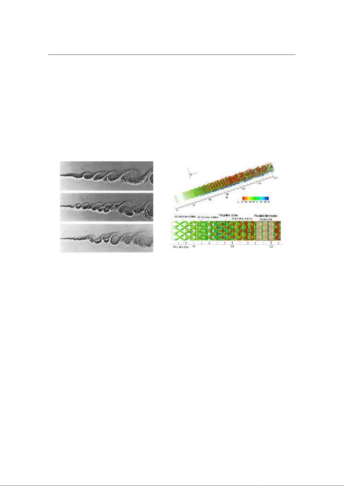
TML has been studied through both experimental and numerical methods. In 1974,
Brown and Roshko [6] observed large vortex structures in Kelvin-Helmholtz vortices.
These vortices formed and moved downstream of the interaction region (Fig. 1a) with the
size of the vortices increasing. According to Kolmogorov's Turbulence Theory [7, 8],
* Corresponding author, email: dungnt42ncs@lqdtu.edu.vn
DOI: 10.56651/lqdtu.jst.v19.n03.813
Journal of Science and Technique - Vol. 19, No. 03 (Nov. 2024)
58
turbulent flow consists of a broad range of eddy sizes, where large-scale structures are
the main carriers of flow energy. Kinetic energy is transferred from larger eddies to
smaller ones and dissipated or converted into heat due to the effect of molecular
viscosity. Recognizing that large-scale structures are key to explaining the behaviors of
the mixing layers, further studies have focused on describing these large-scale
structures. Many studies on large-scale structures using different methods, including
experimental (Exp), direct numerical simulation (DNS), and large eddy simulation
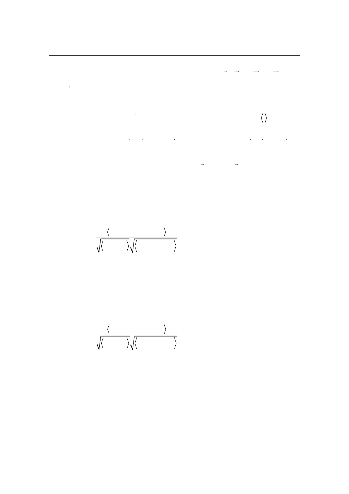
(LES), are summarized in Table 1. Various types of structures in the mixing layers are
shown in Fig. 1b.
(a)
(b)
Fig. 1. The large-scale structures in the mixing layers
(a) Shadowgraphs of mixing layer by Brown and Roshko, 1974 [6];
(b) Visualization of eddy structures by Zhang et al., 2019 [9].
Durbin highlighted in his book that the turbulence problem is not a matter of
physical law, but rather a problem of description [10]. Analyzing turbulent flow through
numerical or experimental methods inevitably leads to a statistical description.
Typically, this involves a dataset of velocity fields at discrete points in space and at
different times. Due to the statistical and discrete nature of the dataset, methods based
on statistical theory and matrix algebra are particularly suitable for studying turbulent
flow. Townsend pointed out that a notable characteristic of turbulent motion is that it is
less random than chaotic gaseous environments, due to the influence of the pressure
field on the motion of fluid particles [11]. Therefore, when analyzing turbulent flow, in
addition to accurately describing variables at a single point, it is also necessary to
consider the relationship of variables between points in the flow environment.

Tạp chí Khoa học và Kỹ thuật - ISSN 1859-0209
59
Table 1. Summary of the large-scale structures in the shear mixing layers
Research, Year
Method
Results
Brown & Roshko [6],
1974
Exp
- For flow with low Reynolds number the large eddies are two-
dimensional.
- The spacing between vortex rollers increases with increasing
distance downstream.
Sandham & Reynolds
[16], 1991
LES
- Identified the inclined Λ-vortex in the temporal simulations at
MC = 0.8.
Clemens & Mungal
[17], 1995
Exp
- The mixing layer becomes highly three-dimensional with the
increasing convective Mach number MC.
Fu et al. [18], 2000
DNS
- The development of structures in mixing layers goes from the
formation of Λ-vortices, through horseshoe vortices and mushroom
structures to the smaller vortices of the fully turbulent state.
Qibing Li et al. [19],
2003
LES
- Distance for the large-scale vortex development increases with
convective Mach number MC.
Fu & Li [20], 2006
LES
- Oblique structures are more prevalent in the flow with higher MC.
Liu & Chen [21], 2010
DNS
- The ring-like vortices generation is caused by the interaction
between the Λ-shaped vortex tube and streamwise vortices.
- The multiple ring-like vortex generation follows the first
Helmholtz vortex conservation law.
Zhou et al. [22], 2012
DNS
- Λ-vortices, hairpin vortices, and ‘flower’ structures are populated in
the transition process of the flow fields.
- Hairpin vortices play an important role in the breakdown of the flow.
Yang et al. [23], 2019
DNS
- The large-scale structures in the subsonic-supersonic shear
mixing layers formed the small structure earlier.
- The Λ eddy and hairpin eddy can be observed, and Λ eddy
structure is elongated with the increase of Mc.
Zhang et al. [9], 2019
DNS
- The presence of multiple ring-like vortices leads to local strong
ejection and sweep regions.
- The appearance of multiple ring-like vortices and their evolution
can significantly promote mixing in the transition stage.
Chong et al. [24], 2021
DNS
- Multiple necklace-like vortices evolve from the Λ-vortices.
Lars Davidson [12], in his lecture notes, defined the term 'correlation' as the
tendency of two values or variables to change together, either similarly or oppositely.
Additionally, a two-point correlation is analogous to the covariance of two statistical
ensembles. In turbulent flow, two-point correlation encompasses various correlation
coefficients corresponding to different pairs of variables at two points in the spatial

Journal of Science and Technique - Vol. 19, No. 03 (Nov. 2024)
60
domain under investigation. Many kinds of two-point correlation coefficients have been
studied, such as velocity-velocity correlation, velocity-vorticity correlation, and other
correlation conditions used in publications by Sillero and Jimenez [13], Chen et al. [14],
and Hwang [15]. These analytical techniques are used to highlight the behaviors of large-
scale structures in turbulent flow, with characteristics such as shape, size, and position. In
turbulent flow research, two-point statistical correlations are used to determine the
integral length scales of eddie structures, analyze the energy spectrum, and evaluate the
dissipation rate from the perspective of Kolmogorov's Turbulent Theory.
There are two concepts involving two-point statistical correlation: temporal
correlation and spatial correlation. Temporal correlation, also known as autocorrelation,
essentially considers the correlation of two variables at the same location but at different
times. The temporal correlation coefficient is used to determine the integral time scale,
while the spatial correlation coefficient is used to determine the integral length scale and
energy spectrum.
In this article, the authors focus on using two-point correlation to study large
structures in the mixing layers. We specifically employ the spatial correlation
coefficients of two variables at distinct locations to determine the length scale, assess
changes in the size of vortices, and define the energy spectrum. While Kim et al. also
used this method to study large vortex structures in 2020 [25], their focus was limited to
vortex structures in the self-similar region. In contrast, we chose to investigate both the
transition region and the self-similar region, allowing us to evaluate changes in large
vortex structures from the initial stage to the point when the flow reaches a fully
turbulent state.
The experimental data used for the calculations in this paper were sourced from
the publication by Kim et al. [26], specifically the SPIV velocity field data, which is
accessible online. The calculations in this study were performed using algorithms and
MATLAB code developed by the authors themselves. The results provide analyses and
evaluations of turbulent organization, enhancing the understanding and knowledge of
turbulent mixing layers.
2. Computational method
2.1. Two-point correlation
We use the two-point correlation function presented by Pope [27] in his book
as follows:
( , ) , ( , )
ij i j
R r t u r t u r r t
(1)
Tạp chí Khoa học và Kỹ thuật - ISSN 1859-0209
61
where ui, uj (i, j = 1, 2, 3) denote the velocity fluctuations;
1 2 3
r e x e y e z
and
rr
are reference location vectors for two distinct points; the numbered indices
(i, j = 1, 2, 3) respectively indicate the streamwise (x-direction), transverse (y-direction)
and spanwise (z-direction);
i
e
denote the unit vector of the i-direction;
denote an
ensemble average. There are one-dimensional spatial correlation and two-dimensional
spatial correlation, with
1
r e x
or
2
r e y
for the first,
12
r e x e y
and for the other. When using notation without numerical indices, the velocity
fluctuation vector can be understood in the form
1 2 3
, , ( , , ).u u v w u u u u
Note that
some documents use u', v', and w' to denote velocity fluctuation components.
One-dimensional spatial correlation is used to define the size of the largest eddies
in the turbulent field, it is useful to call integral length scale. If two points are located in
the x-direction, the correlation is called the longitudinal correlation coefficient
22
, ( , )
( , ) ( , )
uux
u x y u x x y
C
u x y u x x y
(2)
and the longitudinal integral length scale for components of velocity u-u:
0
()
uux uux
L C x dx
(3)
Similarly, we can define the transverse spatial correlation coefficient and the
transverse integral length scale for components of velocity u-u.
22
, ( , )
( , ) ( , )
uuy
u x y u x y y
C
u x y u x y y
(4)
0
()
uuy uuy
L C y dy
(5)
By substituting the u-u velocity components with v-v velocity components in
expressions from (2) to (5), we can define Cvvx, Cvvy, Lvvx, and Lvvy for the variable pair
of v-v velocity components.


![Giáo trình Cấu trúc dữ liệu và giải thuật - Trường CĐ Cơ điện Hà Nội [Mới nhất]](https://cdn.tailieu.vn/images/document/thumbnail/2026/20260323/lionelmessi01/135x160/58171774381670.jpg)


![Giáo trình Tiện nâng cao (Nghề Cắt gọt kim loại, Trình độ Cao đẳng) - Trường Cao đẳng Cơ điện Hà Nội [Mới nhất]](https://cdn.tailieu.vn/images/document/thumbnail/2026/20260323/lionelmessi01/135x160/48101774403543.jpg)


