
HPU2. Nat. Sci. Tech. Vol 02, issue 01 (2023), 25-37
HPU2 Journal of Sciences:
Natural Sciences and Technology
journal homepage: https://sj.hpu2.edu.vn
Article type: Research article
Received date: 10-4-2023 ; Revised date: 24-4-2023 ; Accepted date: 24-4-2023
This is licensed under the CC BY-NC-ND 4.0
On the puiseux theorem
Minh-Tam Dinh Thi*
K45- Math - English pedagogy, Hanoi Pedagogical University 2, 32 Nguyen Van Linh, Phuc Yen, Vinh Phuc,
Vietnam
Abstract
In 1850, Puiseux solved the problem of finding roots of complex polynomials in two variables and
proved that the field of these series is algebraically closed. His proof provided an algorithm
constructing the roots.
In this article, based on the paper “Ha Huy Vui, Nguyen Hong Duc. On the Lojasiewicz exponent near
the fibre of polynomial mappings, Ann. Polon. Math. 94 (2008), 43-52”, we give a different algorithm
computing Newton - Puiseux roots of a complex polynomial in two variables. This algorithm is more
effective in practice.
Keywords: “the Puiseux Theorem”, “the Puiseux theorem”.
1. Introduction
As a continuation of the classical problem of finding all roots of a complex polynomial, Puiseux
Theorem gives an algorithm looking for roots of polynomial in two variables. It quickly became a
powerful tool in many areas of mathematics such as algebra, semi-algebraic, number theory. Let
( , ) [ , ]f x y x y
be a complex polynomial. We may consider
( , ) C[ ][ ]f x y x y
as a polynomial of
one variable
y
with coefficients in the ring
[]x
. A classical problem in mathematics is to find roots
of
f
. In [1], [3], [4], Puiseux gave an algorithm finding all roots
( )
i
y y x=
of
( )
,0f x y =
. In this
article based on [2], we give a different algorithm computing the roots
( )
i
yx
. This method is easier
in practice as Example 4.5, 4.6, 4.7 illustrated. The article is organized as follows.
* Corresponding author, E-mail: minhtam19521@gmail.com.
https://doi.org/10.56764/hpu2.jos.2023.1.2.25-37
HPU2. Nat. Sci. Tech. 2023, 2(1), 25-37
https://sj.hpu2.edu.vn 26
1. We will present overview about the Puiseux series.
2. The next part of the article, we give an inductive algorithm, named the Newton - Puiseux
algorithm, which gives all
y
-roots of
f
. Recall the definition of the Newton polygon of
f
and give
some examples to represent them on diagram.
3. In last section, we will give the main result of the paper which is Puiseux's theorem.
2. Puiseux series
Let
1
[[ ,..., ]]
n
xx
be ring of formal power series.
Definition 2.1. A Puiseux series over is a series of the form:
12
//
12
( ) ...,
n N n N
a x c x c x
= = + +
where
1 1 2
0, , , , ..., 0.
ii
c c n N n n N
Let
1/nN
be called the order of
and denoted by
ord( )
.
The ring of Puiseux series over is denoted by
x
.
Assume that
12 /
//
12
1
( ) . ,.. i
nN
n N n N
i
i
x c x c x c x
= + + =
and
12 /
//
12
1
( ) . ,.. i
mM
m M m M
i
i
x b x b x b x
= + + =
are any two Puiseux series. The addition, multiplication operations in
x
are defined as the
polynomial rings.
Remark 2.2. We see that
12
12
( ) ... [[ ]]
nn
N
y c y c y x
= + +
.
Lemma 2.3.
( )
,,x +
is a field.
Proof. We only need to prove that for all
(0) 0
then
()x
is invertible, i.e, there exists
()xx
such that
( ). ( ) 1xx
=
.
Assume that
12
//
12
( ) ...,
n N n N
x c x c x
= + +
where
1 1 2
, 0, , , ..., 0.
ii
c c n N n n N
Let
1/ N
yx=
where
N
is the common denominator of all exponents in the Puiseux series. Then
( )
12
1 2 1
1
12
12
( ) ( ) ... [[ ]]
...
( ).
nn
N
n n n
n
x y c y c y x
y c c y
yy
−
= = + +
= + +
=
We have
1
(0) 0c
=
. Then there exist
( ) [[ ]]yx
such that (proved in Lemma 2.4).
Define
1/1/
( ) ( )
nN N
x x x
−
=
.
Then,
HPU2. Nat. Sci. Tech. 2023, 2(1), 25-37
https://sj.hpu2.edu.vn 27
11
/1/
( ). ( ) ( ). ( ) ( ). ( ) 1.
n n N
N N N
x x y y y y x x
−
= = =
Lemma 2.4. Let
( ) [[ ]]xx
such that
(0) 0
. Then
is invertible.
Proof. Let
[[ ]]x
be the ring of formal power series and let us write
()x
as
0 1 0
..., 0a a x a+ +
and
()x
as
01...b b x++
. We will inductively construct a series
()x
satisfying
( ) ( ) 1xx
=
. We have:
2
0 0 0 1 1 0 0 2 1 1 2 0
01
( ) ( ) ( ) ( ) ...
... ... 1.
n
n
x x a b a b a b x a b a b a b x
c c x c x
= + + + + + +
= + + + + =
Then
0
0
1
ba
=
and
10 1
12
00
,...
ab a
baa
= − = −
Assume that we have obtained
0,..., n
bb
such that
01
1, ... 0.
n
c c c= = = =
We defined:
1 1 0
1
0
... .
nn
n
a b a b
ba
+
+
++
=−
Then
0 1 1 1 0
... 0.
n n n
a b a b a b
++
+ + + =
Hence, there exists
()x
such that
( ) ( ) 1xx
=
.
3. Newton polygon
In the section, we will present an inductive algorithm, named the Newton - Puiseux algorithm,
which gives all
y
-roots of
f
.
Consider
( )
, [[ ]]f x y x y
and
( )
( )
,
, ( ) n
n
f x y c x y c x y
==
.
Definition 3.1. Let
( )
Supp( ) : , 0fc
=
be the support of
f
.
Let
()f
−
be convex hull of the set
( ) ( )
2
, , Supp( )f
+
+
.
Let
f
be the union of compact edges of
()f
−
, we call it the Newton polygon (diagram) of
f
.
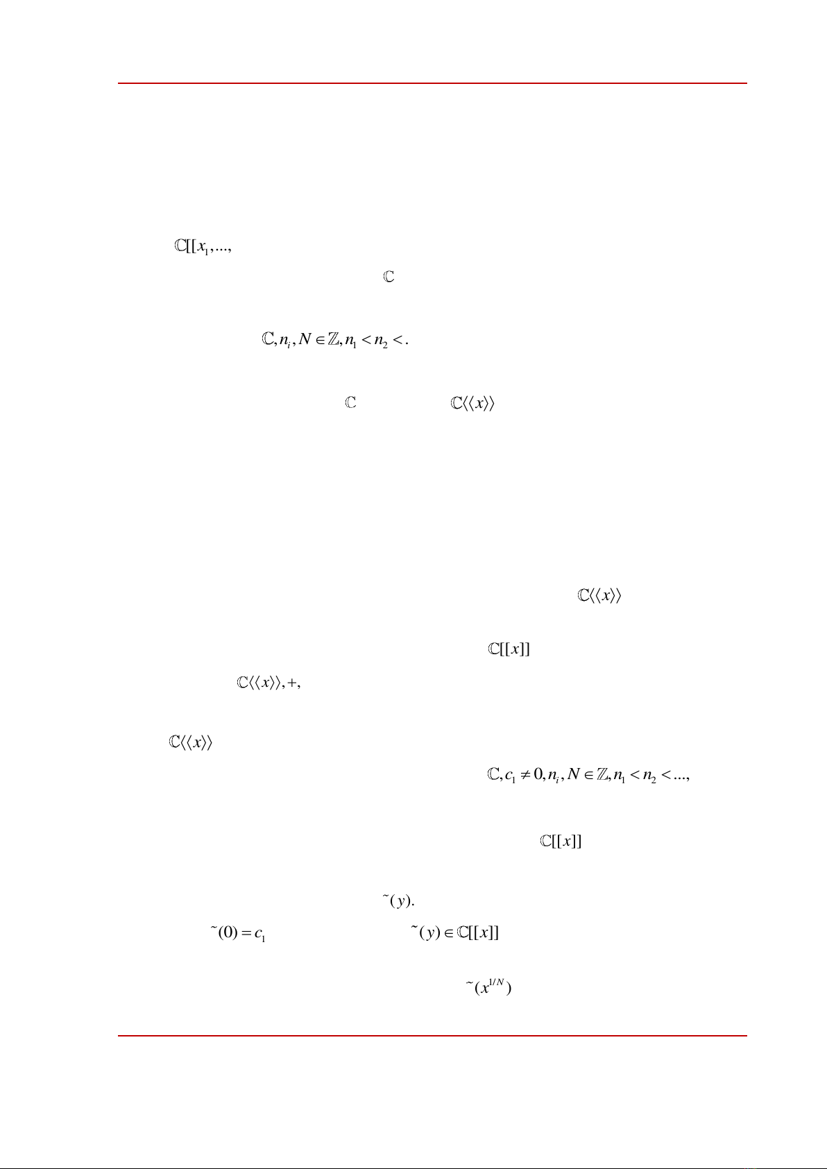
Example 3.2. Let
( )
2 4 1/2 3 2/3 5 3
, 3 7f x y x y x y x y x y
−
= − + + +
.
We have:
( ) ( ) ( )
12
( ) 2;4 , ;3 , ;5 , 3;0 , 0;1
23
f
−
= −
.
HPU2. Nat. Sci. Tech. 2023, 2(1), 25-37
https://sj.hpu2.edu.vn 28
f
is the polylines connecting the points
( )
1;3 , 0;1
2
−
and
( )
3;0
.
Figure 3.1. The Newton polygon of
f
.
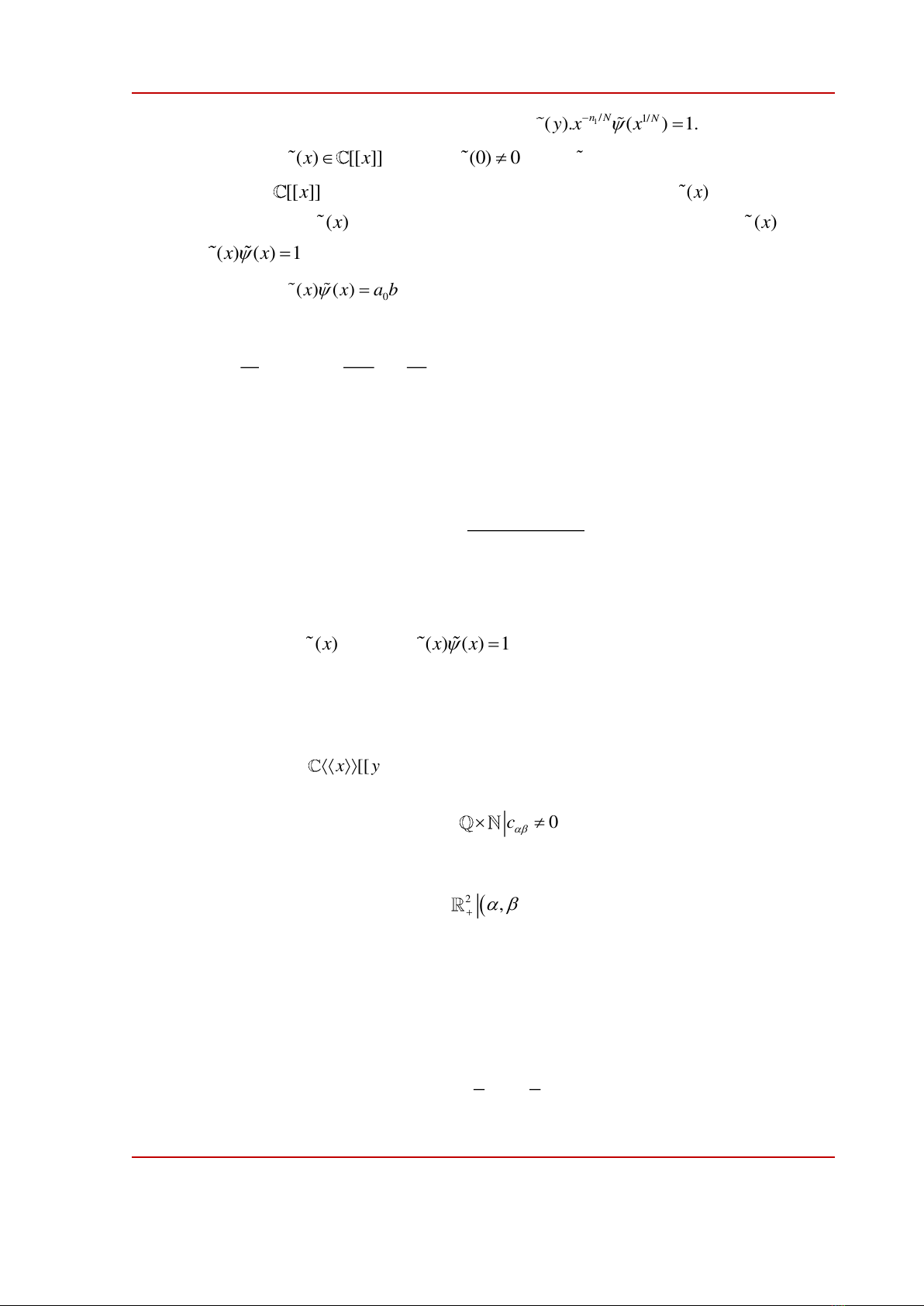
Example 3.3. Let
3 1/2 5 3/5 2
( , ) 2 5f x y xy x y x y x
−
= − + +
.
We have:
( ) ( )
13
( ) 1;3 , ;5 , ;1 , 2;0
25
f
−
−
=
.
f
is the polylines connecting the points
13
;5 , ;1
25
−
and
( )
2;0
.
Figure 3.2. The Newton polygon of
f
.
4. Main result
In this section, we state the Puiseux Theorem saying that the field of Newton - Puiseux series is
algebraically closed. Equivalently, one can find the roots of the equation
( )
,0f x y =
in the form
( )
y y x=
where
( )
yx
are Puiseux series. This has proven in [3], [4]. The proof provide an
algorithm to find the roots
( )
y y x=
of
( )
,0f x y =
. We introduce a new algorithm also computing
the roots of the equation. It based on the “sliding method” introduced in [5] and developed in [2].

HPU2. Nat. Sci. Tech. 2023, 2(1), 25-37
https://sj.hpu2.edu.vn 29
Theorem 4.1. (Puiseux) Let
[[ , ]]f x y
such that
ord (0, )f y m=
then
( )
1
( , ). ( )
m
i
i
f u x y y y x
=
=−
,
where
( )
,u x y
is invertible in
[[ , ]]xy
and
()
i
yx
is Puiseux series in
x
. The series
()
i
yx
are called Newton - Puiseux roots of
f
.
Corollary 4.2. The field
x
is algebraically closed.
We will not prove the theorem but we will give an algorithm for constructing the solution
()sx
.
The algorithm is based on the paper [2], [5]. The algorithm as follow:
,
,
()f x c x y
=
.
- The first step: Construct
1
E
P ( )y
:
+ Let
f
be the Newton polygon of
f
and let
1
E
be the edge of
f
containing the lowest dot
on
Ox
of
f
.
+ Let
( )
1
1
E,
,E
P ( , )x y c x y
=
and
1
1E
P ( ) P (1, ) 0yy
==
.
- The second step: Find
1
a
and
1
with the following properties:
Let
1
a
be a root of
1
P ( )y
and
11
tan 0
=
where
1
is tangent value of the angle
1
determining by
Oy
and
1
E
.
- The third step: Determine
1
11
( , ) ( , )f x y f x y a x
=+
.
- The four step:
+ Applying the third step, we get
22
,a
and
2
f
.
+ Repeating this work (infinity) many times we obtain a sequence
12
12
( ) ... n
nn
s x a x a x a x
= + + +
with
( )
( )
1
( , ) ,
, ( ) .
n
n n n
n
f x y f x y a x
f x y s x
−
=+
=+
- The final step: We define
( ) lim ( )
n
s x s x=
.
The following lemma gives us an observation that
()sx
would be a root of
f
. The fact that
()sx
is indeed a Newton - Puiseux root of
f
can be found in [1].
Lemma 4.3. One has
1
ord ( ,0) ord ( , ( )) ... ord ( , ( ))
n
f x f x s x f x s x
.
Proof. We need only prove that
1
ord ( ,0) ord ( , ( ))f x f x s x
, i.e.,
1
1
ord ( ,0) ord ( , )f x f x a x
,


![Mã hóa mức vật lý: Phần [Thông tin chi tiết/Hướng dẫn/Tổng quan]](https://cdn.tailieu.vn/images/document/thumbnail/2011/20110425/magiethitham/135x160/kythuattruyensolieu_pdf0118_0701.jpg)

![Tài liệu giảng dạy Vi tích phân A2 [chuẩn nhất]](https://cdn.tailieu.vn/images/document/thumbnail/2026/20260323/hoatudang2026/135x160/54651774420904.jpg)


![Tài liệu giảng dạy Hình học Affine và Euclide [chuẩn nhất]](https://cdn.tailieu.vn/images/document/thumbnail/2026/20260323/hoatudang2026/135x160/52531774414221.jpg)


