INTERNAL MEDECINE JOURNAL OF VIETNAM|NO 22/2021
81
CLINICAL RESEARCH
APPLICATION OF NEURAL NETWORKS IN THE
DIAGNOSIS OF HEART DISEASE
Dao Thanh Tung1, Cao Vo San1
1Vietnam Military Medical University
ABSTRACT
Artificial neural networks, which are an essential tool in Machine Learning, are used to solve many types of
problems in different fields. This article will introduce an application of the artificial neural network model in
the diagnosis of heart disease based on the heart.csv data file. The results show that the built model has
high accuracy in the diagnosis, reaching 90.9%, and the area under the ROC curve is 0.939. Compared
with models built with ROC curves, logistic regression, decision trees, or discriminant analysis, the neural
network model proved superior in diagnosis.
* Keywords: Machine learning; Artificial neural networks; Prediction; Classification.
INTRODUCTION
In recent years, AI - Artificial Intelligence and more
specifically, Machine Learning has emerged as
evidence of the fourth industrial revolution.
One of the models widely used in Machine
Learning is Artificial Neural Networks, in which the
Deep Learning technique proves its superiority
over traditional Machine Learning. In medicine,
many problems have been implemented by AI
applications, including the diagnosis of diseases.
The diagnosis is based on some clinical
information surveyed from a person, the doctor
who makes a diagnosis that he is sick or not. It
performs a classification that ranks a person into
one of the two layers (with disease: 1, no disease:
0). For diagnostic (forecast) or sorting objects,
we can build many models to guess data such as
ROC curve, logistic regression, decision tree, or
distinguished analysis, which helps the diagnosis
be effective. However, we always want to build a
model with the exact forecast rates as much as
possible that would replace people in diagnosis
and automatic prognosis.
In this article, the artificial neural network model
app. was used to diagnose a person with heart
disease or not through the heart.csv data set [3]
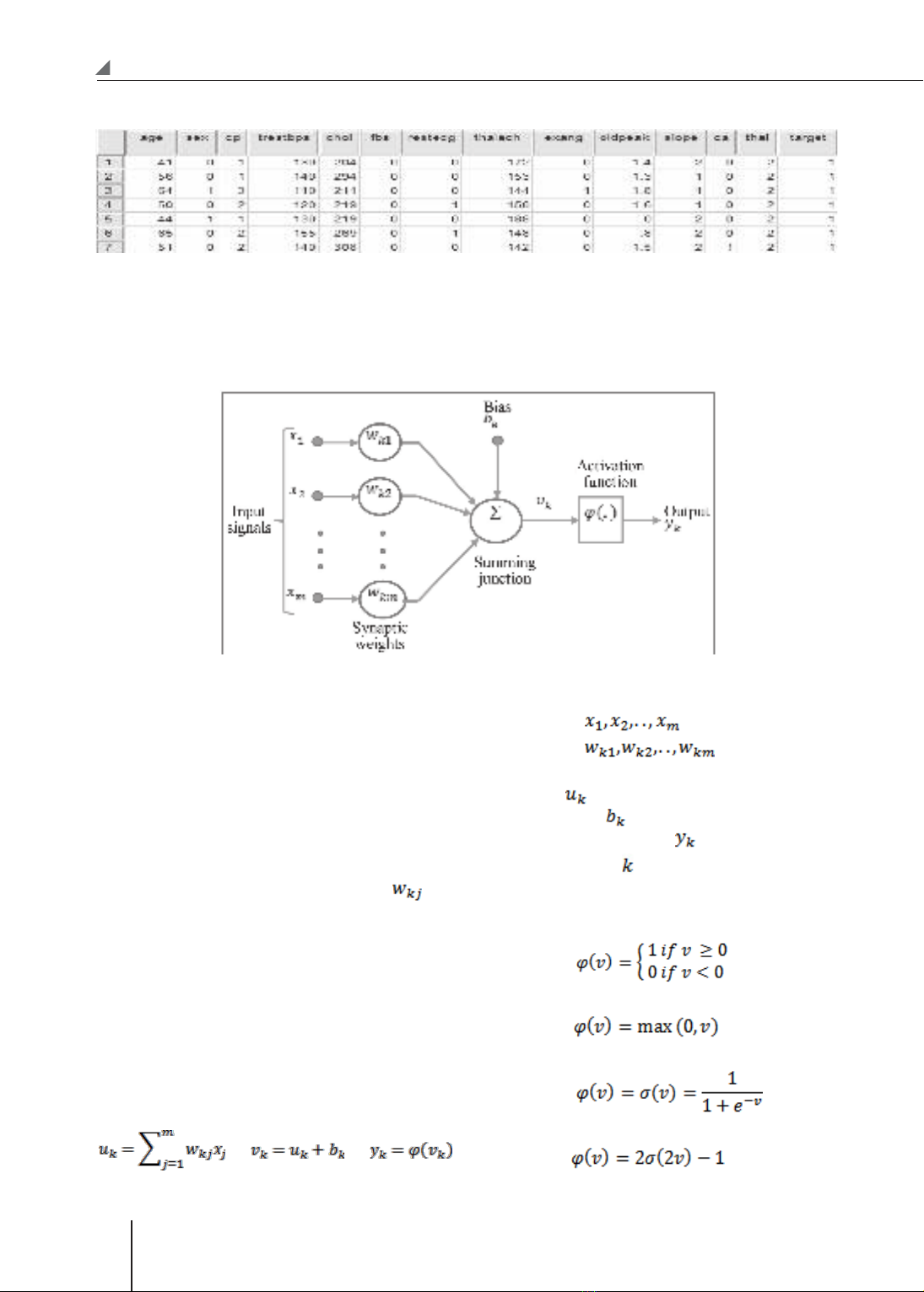
of 303 people, including 165 sick people and 138
healthy people. This data set includes 14 variables:
age (age in years), sex (gender), cp (chest pain
type), trestbps (resting blood pressure (in mmHg on
admission to the hospital), chol (serum cholestoral
in mg/dl), fbs (fasting blood sugar > 120 mg/dl),
restecg (resting electrocardiographic results),
thalach (maximum heartbeat with Thallium Stress
Test), exang (exercise induced angina), oldpeak
(ST depression induced by exercise relative to
rest), slope (the slope of the peak exercise ST
segment), ca (number of major vessels (0-3)
colored by fluoroscopy) , thal (radioactive Thallium
test results) and target (have a disease or not).
Corresponding author: Dao Thanh Tung (daothanhtungk80@gmail.com)
Date received: 10/5/2021
Date accepted: 16/6/2021
INTERNAL MEDECINE JOURNAL OF VIETNAM|NO 22/2021
82
CLINICAL RESEARCH
Figure 1: Part data of the Heart.csv file.
STRUCTURE OF ARTIFICIAL NEURAL NETWORKS
Researchers have sought to understand how biological neurons transform into artificial neural networks,
which can operate on computers.
Figure 2: Model of an artificial neuron.
Figure 2 is a single neuron model, which is
considered the basic information processing unit
of an artificial neural network. A neural network has
three basic components, which are:
- A set of the synapse, also known as connecting
links used to connect the neurons together. A
synapse is used to transmit signals from neurons
labeled j to neurons labeled k with weight .
- An adder is used to synthesize input signals at
each neuron and send a signal to continue.
- An activation function is used to put the output
signals of neurons into a specific domain or a set
of fixed values.
It is possible to describe the operation of neurons
with k in the picture above with the following math
equations:
In which, the are the value of the
input signals, are the weights
corresponding to the synapse link to neurons with
labeling k , is the linear combiner output from
the input signals, is the deviation (bias), φ (.) is
the activation function and is the output signal
from neural labeled
Common activation functions:
- Threshold function
- reLU function (Rectified Linear Unit):
- Sigmoid function:
- Hyperbolic Tangent function:
; ;
are the value of the input signals,
is the deviation (bias), φ (.) is the activation function and
INTERNAL MEDECINE JOURNAL OF VIETNAM|NO 22/2021
83
CLINICAL RESEARCH
- Softmax function
In the classification with k specific layers, the
softmax function used to transfer a k dimensional
vector containing elements - real numbers into a
k-dimensional vector contains elements, which
values are in the range (0; 1):
Each is the probability for input data in the j
layer, and the data is classified into the class that
has the biggest probability.
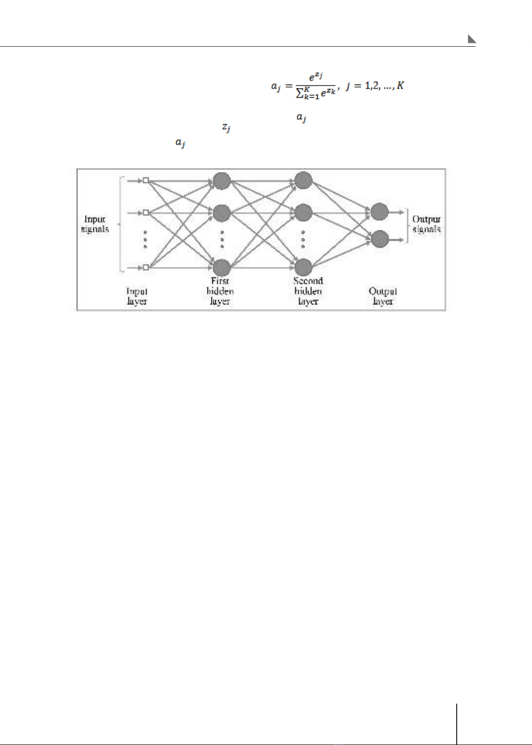
Figure 3: Artificial neural network model.
Neural Networks are formed when we combine
single neurons. In neural networks, neurons
are organized into layers forming a multilayer
perceptron. The first layer on the left is the input
layer, and the last layer on the right is the output
layer, the remaining layers in the middle are hidden
layers. The neurons in a class will have a weight
corresponding to the link to the neurons of another
class. Each neuron in any layer of the network is
connected to all the neurons in the front layer (this
type of connection is called the full connection).
There are no connections between neurons in the
same layer together. The signals are transmitted
in only one direction from left to right via neurons,
and no connections are transmitted in the opposite
direction.
RESULTS OF IMPLEMENTATION ON SPSS
1. Model construction
An essential principle in Machine Learning is the
data split into two parts: Training (Train Data) and
the other used for checking the model (Test Data).
The reason for such division can explain through
the exam preparation. Suppose there are 10 exam
tests. If teaching all ten tests and then take one
of the 10 for testing, most high scores will be
achieved (because they have been learned). But in
fact, when attempting with new data, good results
may not achieve (such a model called overfitting)
since it is just learning without reactivation, unable
to generalize.
In contrast, it could be trained with 8 tests and 2
others for checking the evaluation. After training
on 8 random tests and checked on the remaining
2 tests, if the result is not good, then the score in
the exam with new data is often not good, but if the
test results are good, then the exam will be good.
A typical train/test split would be to use 70% of the
data for training and 30% of the data for testing.
Cases are included in train data or test data
randomly and fully automatically when performing
model building. However, due to the comparison
with other familiar models, the data division is
carried out before but still ensuring randomness
with a group variable.
The form of learning of the model, in this case, is
called supervised learning. The data labeled by
INTERNAL MEDECINE JOURNAL OF VIETNAM|NO 22/2021
84
CLINICAL RESEARCH
experts (doctors): sick or not sick. The model will
mimic professionals estimate the classification
results, match the results of the expert and
gradually adjust the parameters of the model
during the training process.
With usual statistics, the implementations on a
data set, the same result are obtained. But for
machine learning, each training model often gives
a different result. Therefore, it is recommended to
train the model many times and use the model with
the best outcomes. In each time, it is possible to
change some of the following options:
- Type of input data for training: batch (all at once)
or mini-batch (by small part).
- Optimal algorithm: Scaled conjugate gradient or
Gradient descent
- Parameters in training option
- Save the model to the file with the XML format
so that it is possible to use the forecast model
with the new data. The data is only input without
determining the output is sick or not.
- Select the number of hidden layers, units in
each hidden layer, activation function for hidden
layers, and output layers. However, this selection
is possible for the software to perform fully
automatically.
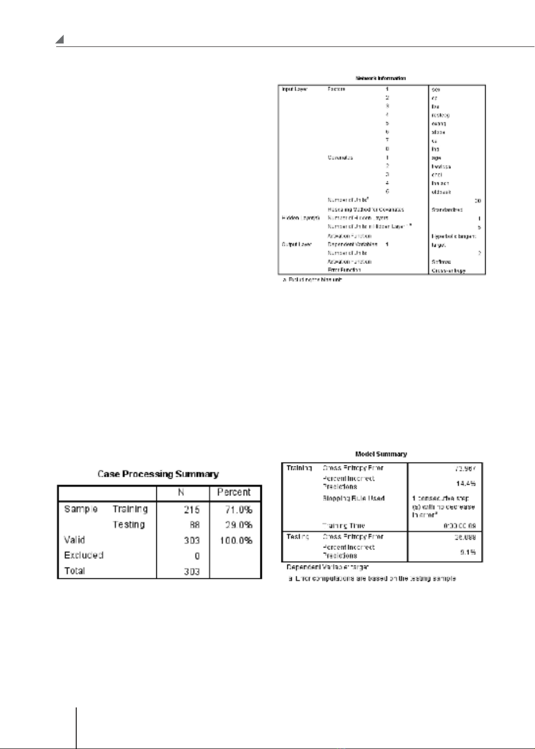
Figure 4: Train data and test data summary table.
Figure 4 shows that training data has 215
cases, equivalent to 71%, and testing data has 88
cases (29%). In each episode, the numbers of sick
or not are unknown because these two episodes
are randomly selected.
Figure 5: Network information results.
The results in figure 5 shows that there are 30
units in the input layer, standardized models,
and the system automatically identified a neural
network model consisting of a hidden layer with 6
units and activation functions hyperbolic tangent.
For the output layer, the dependent variable is the
target variable with 2 output units containing the
probability of classification into the two layers with
the activation function is SoftMax. Loss function or
error function is used as cross-entropy.
Figure 6: Model parameters.
In Figure 6, for the training data, the value of the
error function is 73,967, the not exact forecasting
rate is 14.4%, the stop training rule is a not
descending error function between two times, and
training time only takes 0.09 seconds. For test
INTERNAL MEDECINE JOURNAL OF VIETNAM|NO 22/2021
85
CLINICAL RESEARCH
data, the error function value is 26,088, and the
not exact forecasting rate is only 9.1%.
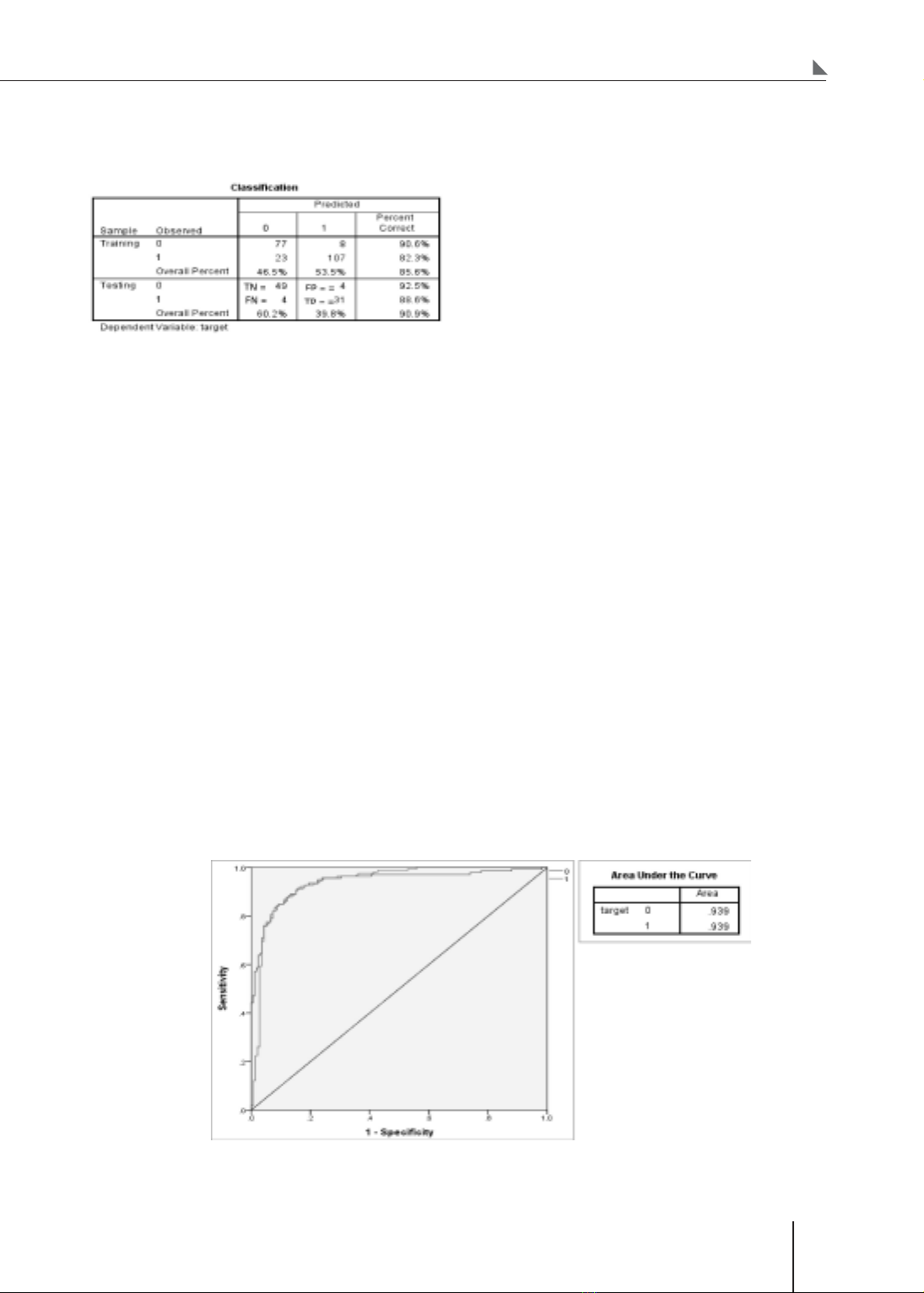
Figure 7: The forecast results of the model on train
data and test data.
The forecast of classification is shown in Figure 7.
Test data has TN = 49 true-negative cases, FP = 4
false-positive cases, FN = 4 false-negative cases
and TP = 31 true-positive cases. Therefore the
basic characteristics in the diagnostic prediction of
the model are:
- Sensitivity: Sens = TP / (TP + FN) = 31 / (31 + 4) =
0.886. That means a person who has disease, and
if let the model makes a diagnosis, the possibility
of the correct conclusion 88.6%.
- Specitivity: Spec = TN/(TN + FP) = 49/(49 +
4) = 0,925. That means a person who has not a
disease, and if let the model make a diagnosis, the
possibility of the correct conclusion is 92,5%.
- Positive Predictive Value: PV+ = TP/(TP + FP) =
31/(31 + 4) = 0.886. That means a person who does
not know is sick or not, and if the model concludes
sick, the possibility of the correct conclusion is
88.6%. The coincidence with the above sensitivity
is random.
- Negative Predictive Value: PV- = TN/(TN + FN)
= 49/(49 + 4) = 0.925. That means a person who
does not know is sick or not, and if the model
concludes not sick, the possibility of the correct
conclusion is 92.5%.
- Predictive value: PV = (TN + TP) / N = (49 + 31)
/ 88 = 0.909. It means that a person who does not
know is sick or not, and if let the model diagnose, the
possibility of giving the correct conclusion is 90.0%.
As we see, the predictive values (also the correct
diagnostic rate or the accuracy of the model)
are essential for a diagnostic model because we
always have to predict for people who do not know
if it is sick or not.
Thus, the above result shows high precision
forecasts in both train data sets and test data.
Hence, the achieved model is good because of the
correct forecast ratio on very high test data sets
and can be trusted when using the model to predict
new data sets. In other words, if there is data on a
person whom an expert has not concluded being
sick or not with heart disease, the diagnostic model
is correct to reach up to 90.9%. The ROC curve of
both layers goes close to the upper left corner with
an area under the curve up to 0.939.
Figure 8: ROC curve and area table under ROC curve.