BỘ GIÁO DỤC VÀ ĐÀO TẠO
VIỆN HÀN LÂM KHOA HỌC VÀ CÔNG NGHỆ VIỆT NAM
HỌC VIỆN KHOA HỌC VÀ CÔNG NGHỆ -----------------------------
Trần Thị Thái
NGHIÊN CỨU MỘT THIÊN HÀ THẤU KÍNH HẤP DẪN CÓ ĐỘ DỊCH
CHUYỂN ĐỎ Z=0.7 SỬ DỤNG DỮ LIỆU ALMA
Chuyên ngành: Vật lý nguyên tử và Hạt nhân
Mã số: 8 44 01 06
LUẬN VĂN THẠC SĨ VẬT LÝ
Hà Nội – 2020
MINISTRY OF EDUCATION
VIETNAM ACADEMY OF SCIENCE AND TECHNOLOGY
GRADUATE UNIVERSITY OF SCIENCE AND TECHNOLOGY -----------------------------
Tran Thi Thai
ALMA OBSERVATIONS OF A GRAVITATIONALLY LENSED GALAXY
AT REDSHIFT z=0.7
Major: Atomic Physics and Nuclei Physics
Number: 8 44 01 06
MASTER THESIS
Supervisor: Dr. PHAM TUAN ANH
Ha Noi – 2020
iii
Acknowledgements
First of all, I would like to express my sincere gratitude to my supervisor Dr Pham Tuan Anh: his constant support, guidance and overall insights in this field made this an inspiring experience for me. I would like to thank Prof. Pierre Darriulat for his continued support throughout this thesis, without his help and wise guidance the thesis would have not been possible.
Furthermore, I would like to thank the rest of the research team in the Department of Astrophysics (DAP) of the Vietnam National Space Center, Ass. Prof. Pham Ngoc Diep who helped me with joining the master course of the Graduate University of Science and Technology; Dr Pham Tuyet Nhung, Dr Do Thi Hoai, Dr Nguyen Thi Phuong and Dr Nguyen Thi Thao have been continuously encouraging me and always willing to help since I joined the team two years ago.
We are deeply grateful to Professors Frederic Courbin and Matus Rybak who kindly provided us with documentation related to the results of the P18 analysis.
The thesis uses ALMA data 2013.1.01207.S (PI: Paraficz Danuta); ALMA is a partnership of ESO (representing its member states), NSF (USA), NINS (Japan), NRC(Canada), NSC/ASIAA (Taiwan), and KASI (South Korea), in cooperation with Chile. The Joint ALMA Observatory is operated by ESO, AUI/NRAO and NAOJ. The data are retrieved from the JVO/NAOJ portal. We are deeply indebted to the ALMA partnership, whose open access policy means invaluable support and encouragement for Vietnamese astrophysics. Financial support from the World Laboratory, Rencontres du Viet Nam, the Odon Vallet foundation and VNSC is gratefully acknowledged. This research is funded by the Vietnam National Foundation for Science and Technology Development (NAFOSTED) under grant number 103.99- 2018.325. I thank the lecturers at the Graduate University of Science and Technology (GUST).
And my biggest thanks to my family for all the support and
encouragements throughout my life.
iv
Lời cam đoan
Tôi xin cam đoan luận văn này là công trình nghiên cứu của tôi được thực
hiện trong suốt thời gian làm học viên cao học tại Học viện Khoa học và
Công nghệ, Viện Hàn lâm Khoa học và Công nghệ Việt Nam. Kết quả nghiên
cứu ở phần 3 là công trình nghiên cứu của tôi dưới sự hướng dẫn của thầy
hướng dẫn và các đồng nghiệp. Những kết quả này là mới và không trùng lặp
với các công bố trước đó.
Hà Nội, ngày tháng năm 2020
Tác giả
Trần Thị Thái
v
Tóm tắt
Vật lý thiên văn hiện đại là một trong những ngành phát triển nhanh nhất hiện nay trong khoa học tự nhiên với rất nhiều câu hỏi thời sự về bản chất của vật chất tối, năng lượng tối, thang Plank, lạm phát vũ trụ… chưa có lời giải đáp. Những câu hỏi quan trọng này sẽ định hình cho sự phát triển của ngành này trong nhiều chục năm tới. Trong đó, nghiên cứu sự hình thành và tiến hóa của thiên hà đang diễn ra thực sự sôi động, cộng đồng Vật lý thiên văn trên thế giới đang tập trung nhiều nỗ lực trên cả hai phương diện lý thuyết và quan sát để dần xây dựng các mảnh ghép quan trọng vào bức tranh tổng thể này.
Thiên hà hình thành và tiến hóa với thời gian hàng tỉ năm, Vũ trụ hiện nay có tuổi khoảng 14 tỉ năm. Vũ trụ đang giãn nở, các thiên hà ngày càng xa nhau. Các thiên hà có độ dịch chuyển đỏ càng lớn, càng ở xa và có vận tốc dịch chuyển ra xa càng lớn. Bản thân chúng là quá khứ của Vũ trụ ở các thời điểm khác nhau. Mục tiêu chính trong nghiên cứu sự tiến hóa của các thiên hà này là xác định các đặc tính của thành phần khí của chúng phụ thuộc theo hàm của độ dịch chuyển đỏ. Từ đó giúp chúng ta hiểu rõ hơn về sự hình thành và tiến hóa của các thiên hà thời kì đầu của Vũ trụ.
Luận văn trình bày nghiên cứu một thiên hà chứa quasar, RX J1131 sử
dụng các quan sát của ALMA ở vạch phát xạ CO(2-1).
Nội dung luận văn gồm 3 phần: Phần đầu tiên: Giới thiệu chung về đối tượng nghiên cứu chính của luận văn, thiên hà chứa quasar RX J1131. Quasar có độ dịch chuyển đỏ zs ~0.65 được quan sát nhờ hiệu ứng thấu kính hấp dẫn mạnh gây bởi một thiên hà chắn giữa có độ dịch chuyển đỏ zL ~0.3. Độ dịch chuyển đỏ của quasar tương ứng với khoảng cách ~1.45 Gpc, hay ~7.5 tỉ năm sau vụ nổ Big Bang, ở thời điểm khoảng một nửa tuổi vũ trụ hiện nay. Thiên hà này chứa một hố đen siêu nặng ở tâm, ~ 2.108 khối lượng Mặt Trời, quay rất nhanh cỡ một nửa vận tốc ánh sáng. Quasar này là đối tượng được quan tâm nghiên cứu đặc biệt nhằm tìm hiểu các thông số vũ trụ học chi phối sự giãn nở của Vũ trụ. Những quan sát về đối tượng này đã được thực hiện trên nhiều hệ kính khác nhau và ở nhiều bước sóng khác nhau như: Kính thiên văn không gian Hubble (trong vùng quang học/hồng ngoại gần), hệ Plateau de Bure Interferometer, hay hệ giao thoa Atacama Large Millimeter/submillimeter Array (ALMA)… Dữ liệu nghiên cứu trong luận văn được lấy từ đài thiên văn ALMA đặt tại sa mạc Actacama, ở độ cao trên 5000m so với mực nước biển, Chile. Đây là một trong những nơi khô nhất trên Trái đất, có điều kiện lí tưởng nhất cho quan sát thiên văn. Chỉ có hai nơi khác trên Trái đất có điều kiện quan sát tốt tương tự: ở đỉnh Maunakea và ở Cực Nam.
vi
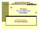
Hình 1: Phổ phát xạ vạch CO(2-1) từ kết quả công bố của Paraficz. Hình trên bên trái: hình ảnh phân bố cường độ sáng trên mặt phẳng trời; hình trên bên phải: phổ vận tốc thể hiện rõ sự bất đối xứng, kết quả của khuếch đại thấu kính hấp dẫn khác nhau với các phần khác nhau của thiên hà; hình dưới bên trái: phân bố vận tốc Doppler trung bình chỉ ra sự biến thiên vận tốc cắt ngang vòng Einstein, dấu hiệu thiên hà đang quay; hình dưới bên phải: hình ảnh phân bố phân tán vận tốc chỉ ra sự không trùng khớp, một trong các kết quả quan trọng đã nêu. Phân bố cường độ bức xạ liên tục được vẽ kèm ở tất cả các hình bằng các đường contour.
Nhóm của giáo sư Paraficz Danuta đã sử dụng dữ liệu thu được từ đài thiên văn ALMA để nghiên cứu hình thái động học của thiên hà này. Đây là bộ dữ liệu có chất lượng rất tốt trong hướng nghiên cứu các thiên hà thấu kính hấp dẫn ở xa. Độ phân giải không gian ~ 0.4 arcsec, độ phân giải vận tốc ~20 km/s, tỉ số tín hiệu so với nhiễu ~ 60 với bức xạ liên tục. Chúng được phân tích chi tiết và công bố bởi nhóm đề xuất quan sát (sau đây gọi là P18). Các kết quả này lần lượt được so sánh và đánh giá cùng với các kết quả của chúng tôi ở phần sau. Một điểm đáng chú ý mà nhóm tác giả đã chỉ ra sự trùng hợp của đỉnh phân bố cường độ sáng trên mặt phẳng trời (sky plane) và vùng có phân tán vận tốc lớn. Nhóm trên gợi ý rằng vùng này gắn với hoạt động hình thành sao của thiên hà.
vii
Phần 2: Trình bày về cách tiếp cận nghiên cứu. Giống như các thiên hà ở xa, quasar này được quan sát nhờ vào hiện tượng thấu kính hấp dẫn. Ảnh thu được của thiên hà này ngoài việc được khuếch đại còn bị biến dạng. Có hai đường cong quan trọng trong nghiên cứu thiên hà thấu kính hấp dẫn: đường caustic nằm trên mặt phẳng nguồn và đường critical curve nằm trên mặt phẳng ảnh. Khi nguồn nằm ở bên trong đường caustic sẽ có 4 ảnh được tạo ra, khi nguồn nằm ngoài đường caustic chỉ có 2 ảnh. Có rất nhiều thiên hà thấu kính được phát hiện có cấu hình giống như RX J1131. Với trường hợp hiện tại, thiên hà này nằm ở vị trí gần với đỉnh (cusp) trên trục chính của caustic. Vị trí của thiên hà thấu kính và của các ảnh được quan sát đồng thời nhờ đó các tham số của thế thấu kính được xác định một cách chính xác cùng với sai số của chúng. Một trong những mục tiêu quan trọng của chúng tôi là đánh giá sai số của các tham số một cách rõ ràng và chỉ ra các mối tương quan nếu có của các tham số với nhau.
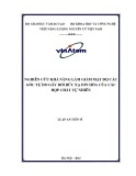
Hình 2: Kết quả mô hình thấu kính hấp dẫn cho nguồn điểm (tâm thiên hà). Sự sai khác giữa ảnh mô hình (dấu cộng màu đỏ) với các ảnh quan sát bởi Kính thiên văn Hubble (dấu cộng màu xanh) chỉ cỡ vài chục so với vài trăm phần nghìn arcsec của các nhóm tác giả khác, chỉ ra sự phù hợp rất tốt mô hình chúng tôi đề xuất. Các đường caustic và đường critical curve được vẽ cùng với vị trí của thiên hà đóng vai trò thấu kính hấp dẫn.
Một kết quả quan trọng khác là các kết luận trong luận văn này độc lập tương đối vào các mô hình thấu kính hấp dẫn (với các chi tiết khác nhau). Thêm nữa, các nghiên cứu tỉ mỉ với độ phân giải góc cao của Kính viễn vọng không gian Hubble (HST) ảnh trong vùng quang học/hồng ngoại gần và của các ảnh Keck Adaptive Optics đã mô tả một cách chi tiết về tính chất của thấu kính trong vùng lân cận của quasar hay tâm của thiên hà. Việc áp dụng mô hình này cho cả một thiên hà với độ bao phủ rộng hơn cả khu vực giới hạn bởi đường caustic là chưa đủ chặt chẽ. Do đó, luận văn đã trình bày chi tiết và đánh giá về sai số liên quan đến việc sử dụng cùng một thế thấu kính cho tâm (nguồn điểm) và toàn bộ thiên hà.
viii
Ở đây, luận văn sử dụng một thế thấu kính mô tả sự bẻ cong:
Hình 3: χ2 trên mặt phẳng (Δx, Δy) (trái), và theo hàm của Δx (giữa), Δy (phải), chỉ ra mối tương quan mạnh giữa hai đại lượng offsets Δx và Δy.
Hình 4: Mối tương quan giữa các tham số của mô hình r0, γ0, rs so với Δx và giữa φo so với φs
ψ=ror+1⁄2γor2cos2(φ–φo) bao gồm 2 thành phần: một thế hình cầu được hiển thị trong thành phần thứ nhất bởi độ manh ro (bán kính vòng Einstein) và một thành phần đặc trưng gọi là shear γo ở vị trí góc φo. Thành phần đầu mô thiên hà thấu kính chính, thành phần thứ hai xét đến đóng góp của các yếu tố khác như: thiên hà vệ tinh, cụm thiên hà, hay những nhiễu loạn nhỏ trong phân bố khối lượng của thấu kính hấp dẫn...Ba tham số (ro, γo, φo) đặc trưng cho thế thấu kính, (Δx, Δy) là offsets nhỏ của tâm thấu kính so với vị trí của thiên hà thấu kính hấp dẫn chính, (rs, φs) ở vị trí của nguồn điểm so với tâm thấu kính.
ix
Hình 3 cho thấy giá trị sai số cuả Δx lớn hơn vài lần Δy. Mối tương quan giữa các đại lượng trong mô hình cũng được chỉ ra ở Hình 4: giữa r0, γ0, rs so với Δx và giữa φ0 so với φs. Luận văn chỉ ra nguyên nhân các tham số này có mối tương quan mạnh do: vị trí của nguồn được xác định so với cusp của caustic, mà không phải với tâm thấu kính. Đại lượng duy nhất phá vỡ tính đối xứng là góc định hướng của shear (do sự xuất hiện của một cụm thiên hà phía đông bắc của thấu kính chính) do đó hệ số góc của mối tương quan φ0 so với φs là 1.
Hình 5: Sự phụ thuộc giữa cường độ sáng của các ảnh (mô hình) khi các tham số của thấu kính được giữ ở giá trị khớp hàm tốt nhất theo hàm của Δx.
Luận văn cũng khảo sát tỉ số cường độ sáng giữa các ảnh A, B, C, D. Kết quả cho thấy, tỉ số A/B, A/C thay đổi không đáng kể, trong khi A/D thay đổi bởi hệ số ~3 khi Δx thay đổi trong khoảng từ –0.2 arcsec đến +0.2 arcsec.
Trong chương này, luận văn trình bày một cách tiếp cận khác với dữ liệu quan sát bởi ALMA và nhắc lại rằng dữ liệu đang được sử dụng có chất lượng hình ảnh tốt nhất từ trước đến nay, kích thước beam quan sát ~0.4×0.3 arcsec2. Nhóm tác giả P18 đã gửi cho chúng tôi các dữ liệu tóm tắt các kết quả chính của họ. Chúng tôi sử dụng một qui trình khác để xử lí dữ liệu thô, có độ phân giải góc tốt hơn nhưng nhiễu cao hơn, qua đó để đánh giá sai số liên quan đến xử lí dữ liệu. Những phân tích trong luận văn này được thực hiện trên mặt phẳng trời (sky plane) thay vì trên mặt phẳng (u,v) giống như P18. Cách làm này cho phép giải thích một cách rõ ràng kết quả thu được ở tất cả các bước. Luận văn chỉ ra những khác biệt giữa cách làm hiện tại với P18 đề cập ở trên không ảnh hưởng gì tới các kết luận của nghiên cứu này.
x
Hình 6: Hàng trên: Phân bố cường độ sáng từ dữ liệu (Jy/beam trái và Jy/pixel giữa) trên mặt phẳng ảnh với dữ liệu của P18 (đường màu đen) và dữ liệu của chúng tôi (đường màu đỏ). Phải: Mối tương quan giữa dữ liệu được xử lí bởi P18 (trục hoành) với dữ liệu của chúng tôi (trục tung), cường độ sáng theo đơn vị Jy/pixel. Hàng giữa và dưới: Phổ vận tốc (Jy) của P18 (đường màu đen) và chúng tôi (đường màu đỏ) lần lượt từ trái qua phải, trên xuống dưới: dữ liệu không cắt, cắt ở 5, 10 ,15 và 20 μJy/pixel.
Luận văn sử dụng hai phương pháp giải ảnh (de-lensing): một trực tiếp (direct-densing) và một thông thường (conventional de-lensing). Ưu điểm của phương pháp trực tiếp là đơn giản và rõ ràng, nhưng nhược điểm là không kiểm soát được hiệu ứng của beam-convolution và cần phải áp dụng ngưỡng cắt dữ liệu mạnh ở mặt phẳng ảnh để tránh de-lensing nhiễu. Trên thực tế, để
xi
Hình 7: Phân bố cường độ sáng của ảnh lấy trung bình cho các khoảng vận tốc (hai cột trái). Bên trái: ảnh quan sát; hình giữa trái: ảnh thu được qua mô hình thấu kính hấp dẫn của chúng tôi từ dữ liệu nguồn của P18, x là trục nằm ngang, y là trục thẳng đứng. Đơn vị của các trục là arcsec. Đơn vị của màu là mJy arcsec–2. Mối tương quan giữa ảnh quan sát và ảnh được giải thấu kính (de-lensing) được chỉ ra ở hai cột phía bên phải. Trục thẳng đứng là cường độ sáng của ảnh quan sát được, trục nằm ngang là cường độ sáng của ảnh thu được từ giải thấu kính. Hình ở giữa bên phải là kết quả của P18, hình bên phải là kết quả của chúng tôi. Các kết quả được hiển thị cho 8 khoảng vận tốc từ xanh nhất tới đỏ nhất từ trên xuống dưới.
áp dụng phương pháp này luận văn sử dụng 1000 điểm ngẫu nhiên cho mỗi pixel có cường độ sáng vượt quá ngưỡng nhất định cho trước và lấy trung bình trọng số phù hợp cho từng pixel nguồn.
Để lấy trung bình trọng số này trước hết cần biết với mỗi pixel ảnh nó được tạo ra bởi nguồn cho hai ảnh (ngoài caustic) hay nguồn cho bốn ảnh
xii
(trong caustic). Với trường hợp đầu trung bình trọng số sẽ cho phân bố cường độ sáng phía ngoài đường caustic và với trường hợp sau là phía trong. Quá trình này cần phải thực hiện thành hai bước độc lập.
Với phương pháp giải ảnh trực tiếp, luận văn sử dụng 125 × 125 pixel ảnh, kích thước 50 × 50 mas2 và dùng ngưỡng cắt 2.4 mJy/arcsec2 mỗi pixel. Trên mặt phẳng nguồn 25 × 25 pixel, 120 × 120 mas2 kích thước mỗi pixel. Kết quả được trình bày ở Hình 8.
Hình 8: Từ trái sang phải: kết quả của P18, của phương pháp giải ảnh trực tiếp, của phương pháp bình phương tối thiểu; từ trên xuống dưới: hình ảnh phân bố cường độ sáng của nguồn phát xạ, hình chiếu cường độ sáng của nguồn lên trục chính của hình ellip trên mặt phẳng trời (sky plane), vận tốc Doppler trung bình.
Phương pháp thứ hai nhằm khắc phục nhược điểm không kiểm soát được hiệu ứng của beam convolution của phương pháp thứ nhất. Từ mô hình phân bố cường độ sáng ban đầu, quá trình tạo ảnh qua thấu kính hấp dẫn diễn ra sau đó, rồi smear ảnh bằng tích chập với beam cho trước rồi so sánh với ảnh quan sát. Quá trình lặp lại cho đến khi tìm được mô hình tốt nhất thông qua đại lượng χ2, xác định sự phù hợp giữa mô hình và quan sát. Trên thực tế, luận văn bắt đầu từ phân bố cường độ sáng của nguồn mà nhóm tác giả P18 đã công bố, tiến hành tinh chỉnh nhỏ cho từng pixel nguồn để tìm cực tiểu của χ2 cho từng khoảng vận tốc. Ở đây độ rộng vạch phổ được chia thành 8 khoảng vận tốc đều nhau, 84 km/s mỗi khoảng. Hình 7 minh họa sự hội tụ của quá trình này và sự phù hợp của mô hình với ảnh quan sát được.
Hình 8 hiển thị kết quả sự phân bố cường độ phát xạ trên mặt phẳng nguồn từ P18, phương pháp giải ảnh trực tiếp và phương pháp thông thường
xiii
Hình 9: Các bản đồ trên mặt phẳng nguồn và ảnh ở khoảng vận tốc đỏ nhất (khoảng thứ 8 trong tám khoảng đề cập ở trên). Hàng trên: Mặt phẳng nguồn, từ trái qua phải: từ P18, từ phương pháp giải ảnh trực tiếp (de-lensing) và từ phương pháp bình phương tối thiểu. Hàng dưới: mặt phẳng ảnh, từ P18 (trái) và từ quan sát (phải). Vòng tròn màu đen hiển thị vùng có khả năng là thiên hà đồng hành. Vòng tròn màu vàng hiển thị ảnh của vùng vòng tròn màu đen trên mặt phẳng ảnh.
(bình phương tối thiểu). Cả ba bản đồ bức xạ này phù hợp với hình chiếu của một đĩa tròn mỏng lên mặt phẳng sky plane với tâm là quasar (x=–0.49 arcsec, y=–0.005 arcsec). Trục chính của hình ellip nghiêng một góc ~14 o về phía Bắc trục x, khoảng 30o theo phương Tây Bắc (nhóm của Leung và cộng sự cho rằng góc này cỡ 31o). Chúng tôi xác định chiều dài trục lớn và nhỏ cỡ 2.7 và 1.6 arcsec (~19 và ~11 kpc) tương ứng với độ nghiêng của đĩa so với mặt phẳng sky plane là cos– 1(1.6/2.7)=54o phù hợp với giá trị xác định bởi P18. Hình 8 cũng chỉ ra hình chiếu của cường độ sáng của nguồn theo trục chính của hình ellip. Bức xạ thay vì cực đại ở vị trí của quasar lại bị giảm đi rõ ràng. Chúng tôi khẳng định đây không phải là sai sót do phương pháp giải ảnh de-lensing mà kết quả này đã thể hiện ở Hình 1, bức xạ ở vị trí ảnh A bị giảm đi trên bản đồ phân bố cường độ sáng của khí phân tử CO(2-1).
Hình 8 từ phân bố của vận tốc Doppler trung bình cho thấy sự biến thiên vận tốc mạnh dọc theo trục chính của ellip, là kết quả của đĩa tròn đang quay.
xiv
y’=Rsinθcos540
z’=Rsinθsin540
Sự xuất hiện của một thiên hà đồng hành ở vùng có vận tốc đỏ nhất đã được đề cập bởi nhóm tác giả Leung và cộng sự (L17) trước đó. Chúng tôi cũng tìm thấy một vùng phát xạ tăng cường trong khoảng vận tốc đỏ nhất với tâm x~0.8 arcsec, y~0.2 arcsec có khả năng là thiên hà đồng hành như đã đề cập (Hình 9). Vị trí của vùng này bên ngoài đường caustic, vùng này tạo ra hai đốm sáng trên mặt phẳng ảnh, ảnh A (đốm mờ) với độ khuếch đại cỡ 0.5, ảnh B với độ khuếch đại cỡ 4.3. Trong khi vị trí ảnh A có lệch khỏi vùng ảnh do đĩa thiên hà tạo ra, nhưng vùng ảnh B hoàn toàn phù hợp. Thêm nữa, đóng góp của hai vùng này trên mặt phẳng nguồn là như nhau và có cùng vận tốc quay với thiên hà chính. Do đó, đây không thể là một thiên hà đồng hành giống như các tác giả trước đã đề cập mà chỉ là một vùng phát xạ tăng cường.
Phần 3: Trình bày những kết quả nghiên cứu chính của luận văn. Ở chương trước, luận văn đã chỉ ra rằng, việc sử dụng một thế thấu kính đơn giản không ảnh hưởng gì nhiều đến sự phân bố cường độ sáng trên mặt phẳng nguồn và phân bố vận tốc Doppler, một đặc trưng của một đĩa mỏng, quay, nghiêng so với mặt phẳng trời (sky plane). Để minh họa tốt hơn (Hình 10), luận văn sử dụng đĩa quay có cường độ sáng đồng nhất với cách chuyển hệ tọa độ dưới đây: x’=Rcosθ Vx =–V(R)sinθ Vy =V(R)cosθcos540 Vz =V(R)cosθsin540
Trong hệ này, trục x nằm về hướng 16o Tây Bắc, tâm của đĩa là quasar (x,y)=(–0.49, –0.005): x+0.49=x’cos14o–y’sin14o y+0.005=x’sin14o+y’cos14o
Từ các phương trình trên kết hợp với kết quả trình bày ở chương trước, ảnh được tạo ra từ một đĩa có cường độ sáng đồng nhất, tâm đĩa ở quasar, nghiêng một góc 540 so với mặt phẳng trời, bán kính đĩa Rdisc =1.35 arcsec.
Hình 10 (phải) cho thấy vùng phát xạ được xác định trong phần nằm giữa của hai đường ellip, đường E+ ứng với đường ellip ở bên ngoài, đường E– ứng với đường ellip bên trong. Tương ứng với hai giá trị của E là giá trị của lambda, λ=0.5 trên E+ và λ = –0.5 trên E–. Xét một điểm bất kì, trong hệ tọa độ Đề-các, vị trí của điểm đó là (x=rcosω, y=rsinω), hay trong hệ tọa độ cực (r,ω), giờ có tọa độ mới là (λ,ω) với λ=[r–(r++r–)/2]/(r+–r–); trong đó r+ và r– là các điểm có vị trí góc định hướng ω trên hình ellip E+ và E– . Tất cả công việc dưới đây được thực hiện trên hệ tọa độ mới (λ, ω, Vz).
xv
Hình 10: Hệ tọa độ (x’, y’, z’) với tâm ở quasar, x’ dọc theo đường giao giữa mặt phẳng đĩa và mặt phẳng trời, z’ vuông góc với mặt phẳng trời. Giữa, phải: Ảnh của đĩa có cường độ sáng đồng nhất được tạo ra nhờ sử dụng thế thấu kính đơn giản và so sánh với hình ảnh quan sát (phải). Đơn vị của mô hình là tùy ý, đơn vị của dữ liệu quan sát là Jy km s –1 arcsec–2 áp dụng cắt ở 0.67 Jy km s–1 arcsec–2.
Hình 11: Hình chiếu cường độ sáng lên ba trục tọa độ mới theo λ (trái), theo ω (giữa) và theo Vz (phải). Hàng trên so sánh dữ liệu mới không cắt (đen) và với cắt ở 1.6-σ (đỏ). Hàng giữa so sánh dữ liệu P18 không cắt (đen) và với cắt ở 1.5-σ (đỏ). Hàng dưới so sánh dữ liệu mới (đen) và dữ liệu của P18 (đỏ) đã được hiệu chỉnh giảm bởi hệ số 0.8.
Với hệ tọa độ cực mới (λ,ω,Vz) luận văn làm việc trong vùng –0.5<λ<+0.5,
0<ω<360o, –340 xvi rộng 0.05 mỗi khoảng, 18 khoảng của ω độ rộng 20o và 16 khoảng của Vz
rộng ~42 km s–1. Từ đó luận văn xây dựng dữ liệu ba chiều mới từ dữ liệu cũ
(gồm 125×125 pixels trên mặt phẳng bầu trời, diện tích 50×50 mas2 mỗi pixel,
80 khoảng vận tốc Doppler có độ rộng 8.417 km s–1 mỗi khoảng). Luận văn
sử dụng 100 điểm ngẫu nhiên với mỗi pixel trên mặt phẳng trời (sky plane) để
dò và xây dựng lên hệ dữ liệu tạo độ cực ba chiều mới. Luận văn tập trung vào nghiên cứu phân bố cường độ sáng trong vùng
chứa nhiễu (50×50×8.417mas2 km s–1) với |λ|>0.5 trên tập dữ liệu do chúng tôi
xử lí. Giá trị trung bình của phân bố Gauss –0.40 μJy and và σ là 7.2μJy.
Cường độ sáng sau đó được hiệu chỉnh lại bằng cách bù thêm một lượng 0.4
μJy trong khối dữ liệu mới. Khi đó tổng cường độ sáng trong toàn khối dữ
liệu là 1.51 Jy. Chúng tôi cũng thu được giá trị tương đương khi áp dụng cắt ở
11.7 μJy cho mỗi pixel. Điều này tương ứng với 11.7/7.2=1.6 σ (Hình 11,
hàng đầu). Làm tương tự đối với dữ liệu của P18, giá trị offset là –0.25 μJy thay cho
–0.40 μJy. Tổng cường độ sáng của khối dữ liệu là 1.90 Jy và đạt giá trị tương
đương khi áp dụng cắt ở 7.1 μJy trên mỗi pixel. Nhiễu trong dữ liệu của
Paraficz nhỏ hơn so với dữ liệu của chúng tôi nên giá trị cắt lúc này
7.1/4.8=1.5 σ (Hình 11, hàng giữa). Hàng cuối cùng của Hình 11, so sánh
giữa dữ liệu của chúng tôi với dữ liệu của P18 trên các trục tọa độ. Ở đây, dữ
liệu của P18 đã được hiệu chỉnh giảm xuống bởi hệ số 0.8 và hai khối dữ liệu
đều không cắt. Sự sai khác trong bốn khối dữ liệu trên cho phép ước lượng sai
số trong của phép đo ~13 mJy cho mỗi khoảng histogram ở Hình 11. Luận văn sử dụng mô hình đường cong vận tốc quay V(R)=V0(eR/R*–1)/
(eR/R*+1) và một đĩa có cường độ sáng đồng nhất có bán kính Rdisc được làm
trơn bởi phân bố σdisc. Thay vì ước lượng giá trị χ2 qua tổng 20×18×16=5760
các phần tử của khối dữ liệu, tôi nhận thấy rằng việc sử dụng tổng gồm
20+18+16=54 khoảng trong Hình 11 tốt hơn khi tính đến sai số của dữ liệu và
sự đơn giản của mô hình. Luận văn sử dụng sai số chung 10 mJy cho mỗi
khoảng và chia cho số bậc tự do để tính giá trị χ2. Giá trị khớp hàm tốt nhất
cho V0=405 km s–1, R*=0.22 arcsec (1.6 kpc), Rdisc=1.10 arcsec (7.7 kpc) và
σdisc=0.32 arcsec (2.2 kpc). Kết quả là đường cong vận tốc quay dốc hơn so
với P18 và L17. Giá trị khớp hàm tốt nhất cho χ2 ~3. Kết quả (Hình 13) chỉ ra, đường
cong vận tốc không phụ thuộc vào cường độ sáng của đĩa nhưng giữa V0 và
R* , Rdisc và σdisc có mối tương quan mạnh với nhau. xvii Hình 12: So sánh hình chiếu cường độ sáng lên các trục tọa độ giữa quan sát (đường
màu đen) và mô hình với sự vắng mặt (đường màu xanh) và có mặt (đường màu đỏ) của
vùng phát xạ tăng cường. Hình 13: Sự phụ thuộc của χ2 vào các tham số mô hình, có tính đến vùng phát xạ, theo R*
và V0 (hàng trên) và theo σdisc và Rdisc (hàng dưới). Theo mỗi cặp kết quả hiển thị cho
trường hợp vắng mặt và có mặt của vùng phát xạ tăng cường gần với quasar. Cho mỗi hàng
các tham số khác được đặt ở các giá trị khớp hàm tốt nhất. Giá trị của FE hiển thị trong mỗi
hình thể hiện hệ số phát xạ tăng cường. So sánh giữa mô hình và dữ liệu trên các mặt phẳng (λ,ω), (λ,Vz) và (Vz,ω)
được trình bày trong Hình 14. Về cơ bản, có sự phù hợp đáng ngạc nhiên giữa
dữ liệu và mô hình (dù rất đơn giản). Hình ảnh trên mặt phẳng (Vz,ω) chỉ rõ xviii Hình 14: Phân bố của hình chiếu cường độ sáng lên các mặt phẳng (λ, ω), (λ, Vz) và (Vz, ω)
và lấy tổng theo trục còn lại theo thứ tự Vz, ω và λ. Đơn vị sử dụng là mJy/bin. Trong các
hình trên, mỗi khoảng theo λ rộng 0.05, theo ω rộng 200, theo Vz rộng 42 km s–1 . Hàng trên
cùng hiển thị ảnh quan sát không áp dụng cắt với dữ liệu. Hàng giữa hiển thị ảnh từ mô
hình khớp hàm tốt nhất. Mô hình (contour) được hiển thị đồng thời trong dữ liệu quan sát ở
hàng trên để tiện so sánh. Hàng bên dưới hiển thị sự khác biệt giữa mô hình và dữ liệu
quan sát. Hai vùng hình chữ nhật (trái) thể hiện rõ nhất sự không đồng nhất của nguồn.
Một trong hai nằm ngay trên đường critical cũng được chỉ ra ở đây (trong hệ tọa độ cực). ràng dấu hiệu của đĩa đang quay. Sự bất đối xứng của phổ vận tốc Doppler
hiển thị trong cả mô hình và dữ liệu quan sát; đây là kết quả trực tiếp của
trường hợp đường caustic nằm ngay trong vùng vận tốc Doppler đỏ của đĩa
quay (phía đi ra xa theo phương nhìn). Hình 12 và Hình 14 cho thấy lợi thế trong việc đánh giá hình thái và động học của thiên hà nguồn mà chưa cần tới việc giải thấu kính (de-lensing). Sự khác biệt rõ nhất giữa mô hình khớp hàm tốt nhất và dữ liệu thể hiện ở
Hình 14 (hàng dưới). Chúng nằm chủ yếu ở hai khoảng (bin) vận tốc Doppler
đỏ nhất và trong vùng tương đối hẹp theo ω, từ 200o tới 240o. Trong mặt
phẳng (λ,ω) vị trí của chúng nằm ở hai hình chữ nhật, E (vùng phát xạ tăng xix Hình 15: Hàng trên: Kết quả của giải thấu kính, sự phân bố cường độ sáng của vùng giảm
phát D, và vùng phát xạ tăng cường E trên mặt phẳng nguồn. Hàng dưới: sự phụ thuộc của
χ2 theo hệ số phát xạ giảm phát FD (trái) và tăng cường FE phải khi các tham số khác của
mô hình được giữ ở giá trị khớp hàm tốt nhất. cường) (200o<ω<235o, –0.18<λ<–0.05) và vùng D (vùng giảm phát)
(207o<ω<237o, 0.15<λ<0.27). Hình 15 (hàng trên) chỉ ra vị trí tương ứng của
chúng trên mặt phẳng nguồn. Kết quả giải thấu kính cho thấy, trên mặt phẳng nguồn, vùng D nằm phía
ngoài đường caustic, độ khuếch đại của vùng này nằm trong khoảng ~3 – 5.
Ảnh đồng hành với D có tâm ở (x,y)~(0.75, 0.25) arcsec và độ khuếch đại nhỏ
nằm trong khoảng 0.5 đến 1. Trong khi đó, vùng E nằm trong đường caustic,
chạm vào cạnh của nó, độ khuếch đại của nó trải rộng trong khoảng từ ~4 đến
vô cùng, độ khuếch đại trung bình cỡ ~20. Có thêm ba ảnh đồng hành với E
với độ khuếch đại trải rộng từ 1.5 đến 5.5. Tâm của một trong ba ảnh ở
(x,y)~(–1, 2) arcsec và vùng này có thể thấy trong Hình 14 (hàng dưới, trái)
nơi dữ liệu nhỉnh hơn một chút so với mô hình. Kết quả của việc giải thấu
kính vùng E cho ra nguồn nằm trong đường caustic không phải là sai sót do
phương pháp. Thực tế nguồn tạo ra vùng E nằm trên và bao phủ về hai phía xx đường caustic nhưng chỉ phần nằm trong của nó đóng góp vào vùng E. Phần
kia tạo ra các ảnh đồng hành của nó, một trong số đó nằm gần vị trí (x,y)~(–1,
2), một ảnh khác nằm gần vùng E. Hình 16: Trái: Sự phụ thuộc của Luận văn đã thử đưa thêm cả vùng phát xạ tăng cường E và vùng giảm
phát D vào mô hình để giải thích cho sự bất đồng nhất của cường độ sáng
giữa mô hình hiện tại và dữ liệu. Trong cả hai trường hợp, giá trị khớp hàm
tốt nhất của các đại lượng V0, R*, Rdisc và σdisc không bị ảnh hưởng. Sự có mặt
của vùng D không cải thiện giá trị của χ2; trong khi đó, vùng E giúp đáng kể.
Giá trị khớp hàm tốt nhất của các đại lượng trong mô hình: V0=435 km s–1,
R*=0.26 arcsec (1.8 kpc), Rdisc=1.10 arcsec (7.7 kpc), σdisc=0.32 arcsec (2.25
arcsec) và FE=2.5. Luận văn cũng đánh giá đường cong vận tốc quay dọc theo trục chính của
hình ellip giống như P18 và L17. Chiều rộng của dải xét trong khoảng độ
rộng ±1 kpc và chiều dài 2.7 arcsec (~19 kpc), chia làm 9 khoảng, mỗi
khoảng có chiều dài 0.3 arcsec (~2 kpc). Trong mỗi khoảng, luận văn so sánh
sự khác biệt giữa mô hình và dữ liệu thu được của phổ vận tốc. Về mặt định
tính, có sự phù hợp giữa mô hình và dữ liệu, tuy nhiên có sự khác biệt đáng
kể ở các khoảng vận tốc trung tâm: dữ liệu cho thấy vận tốc Doppler lớn hơn
ở phía đỏ và thấp hơn ở phía màu xanh so với mô hình. Hơn nữa, trong
khoảng trung tâm, độ rộng phổ từ mô hình nhỏ hơn nhiều so với trong dữ
liệu. Điều này có khả năng là do dạng cong vênh (warping) của đĩa gây ra.
Tuy nhiên việc đưa thêm vào yếu tố này không giúp được nhiều. Điều đó cho
thấy rằng động học của đĩa thực tế phức tạp hơn so với mô hình một đĩa quay
đơn giản của chúng tôi. Luận văn chỉ ra đóng góp quan trọng của thành phần vận tốc quay trong
mỗi chín khoảng nói trên. Điều này dẫn tới đường cong vận tốc quay của
chúng tôi dốc hơn so với P18 và L17. xxi Hình 17: Phổ trong vùng |λ|<0.25, 110o<ω<250o. Hình bên trái là phổ thu được từ quan sát
với cắt ở 11.7 μJy (đen) hoặc 16 μJy (đỏ) với giá trị khớp hàm Gaussian tương ứng σ=85
km s–1 and 56 km s–1. Hình ở giữa và bên phải hiển thị khớp hàm Gaussian lên mô hình
phổ của đĩa với sự vắng mặt và xuất hiện hiệu ứng beam convolution với giá trị σ tương
ứng 18 km s–1 và 58 km s–1. Điểm đáng lưu ý là việc giảm kích thước của mỗi phần tử của khối dữ
liệu ba chiều mới sẽ làm giảm trực tiếp đóng góp của thành phần vận tốc quay
tới độ rộng vạch phổ nhưng không làm giảm đóng góp do hiệu ứng smear khi
tích chập với beam quan sát. Xét khoảng trung tâm của mặt phẳng (λ,θ) trong
vùng |λ|<0.25 và |ω–180o|<70o, gồm 10×14 pixels, mỗi khoảng của λ rộng
0.05, θ rộng 10o. Trong mỗi pixel (i,j) mới này tiến hành xác định giá trị trung
bình Do mô hình không tính đến sự mở rộng vạch phổ do nhiễu loạn
(turbulence) nên sự mở rộng này hoàn toàn do thành phần vận tốc quay. Hình
17 cho thấy đóng góp này cỡ 60 ± 10 km s–1 cho độ rộng vạch phổ. Nó cùng
cỡ với độ rộng vạch phổ quan sát được khi sử dụng dữ liệu cắt ở 2-σ. Tuy
nhiên, khi sử dụng dữ liệu cắt ít hơn, đóng góp của thành phần nhiễu loạn có
thể đáng kể, lên tới ~60 km s–1. Điều này ngăn cản việc ước lượng một cách
tin cậy sự đóng góp của nhiễu loạn cho độ rộng của vạch phổ. Tóm lại, luận văn đã phân tích dữ liệu ALMA bức xạ khí phân tử CO
(2-1) của thiên hà RX J1131, một thiên hà thấu kính hấp dẫn có độ dịch
chuyển đỏ z ~ 0.65. Luận văn so sánh kết quả này với nhóm của những người
đề xuất P18 với mục đích là để đánh giá những sai số kèm theo. Cụ thể, luận
văn sử dụng một quy trình xử lí dữ liệu ALMA khác và mô hình thấu kính
đơn giản hơn so với P18. Luận văn cơ bản khẳng định tính đúng đắn và chắc
chắn của các kết quả trước đó của P18. Luận văn sử dụng hệ tọa độ cực để phân tích dữ liệu, và cho thấy sự
thuận tiện hơn trong việc diễn giải dữ liệu so với hệ tọa độ Đề-các. Nó cho
phép chỉ ra dấu hiệu rõ ràng của một đĩa thiên hà đang quay. xxii Luận văn tìm thấy bằng chứng cho một vùng phát xạ tăng cường ở
khoảng vận tốc đỏ nhất, với hệ số phát xạ tăng cường ~2.5 lần cao hơn so với
mức trung bình. Tuy nhiên vị trí của nó nằm trên đường caustic gây khó khăn
cho việc diễn giải một cách tin cậy về hình thái của nó. Luận văn cho thấy đường cong vận tốc quay dốc hơn so với P18 và
đánh giá đóng góp của thành phần vận tốc này cho độ rộng vạch phổ ~60±10
km s–1, tương đương với độ rộng quan sát khi áp dụng cắt 2-σ trên dữ liệu.
Điều này gây khó khăn cho việc xác định đóng góp của nhiễu loạn một cách
đáng tin cậy, không phù hợp với kết luận của P18. 1 3.2 The data cube.............................................................................................................60
3.3 The disc model...........................................................................................................61
3.4 Brightness inhomogeneity.........................................................................................63
3.5 Rotation and turbulence.............................................................................................66
Summary and conclusions...................................................................................................70
References............................................................................................................................72 2 3 Figure 2.19 Lensing the P18 source brightness distribution................................................57
Figure 2.20 Correlation between observed brightness.........................................................58
Figure 3.1 Geometry in a system of coordinates..................................................................60
Figure 3.2 Projections of the new data cube........................................................................62
Figure 3.3 Comparison between observations and best fit model........................................62
Figure 3.4 Dependence of chisquare on the model parameters............................................63
Figure 3.5 Maps of the brightness projected........................................................................65
Figure 3.6 The brightness distribution in the source plane..................................................65
Figure 3.7 Dependence of mean Doppler velocity on x’.....................................................67
Figure 3.8 Comparison between observed and modelled....................................................68
Figure 3.9 Distributions of the intensity...............................................................................69
Figure 3.10 Line profiles......................................................................................................69 4 5 6 ACA: Atacama Compact Array
ACS: Advanced Camera for Surveys
ALMA: Atacama Large Millimeter/submillimeter Array
AGN: Active Galatic Nucleus
BH: Black Hole
CARMA: Combined Array for Research in Millimeter-wave Astronomy
CASA: Common Astronomy Software Application
CASTLE: CfA- Arizona Space Telescope Lens Survey
DEC: Declination
ESO: European Southern Observatory
FFT: Fast Fourier Transform
FWHM: Full Width at Half Maximum
GILDAS: Grenoble Imaging and Line Data Analysis System
HST: Hubble Space Telescope
HPBW: Half Power Beam Width
IGM: Intergalactic Medium
ISM: Interstellar Medium
L17: Leung et al. 2017
SED: Spectral Energy Distribution
SIE: Singular Isothermal Ellipsoid
SIS: Singular Isothermal Sphere
SMBH: Super Massive Black Hole
SPIRE: Spectral and Photometric Imaging Receiver
PA: Position Angle
PdBI: Plateau de Bure Interferometer
PSF: Point Spread Function
P18: Paraficz et at. 2018
QSO: Quasi Stellar Object
RA: Right Ascension
SFR: Star Formation Rate
SB: Starbust
ULIRGS: Ultra Luminous Infrared Galaxies
VLA: Very Large Array
VLT: Very Large Telescope
WFC: Wide Field Camera 7 1.1 Generalities 1.1.1 RX J1131 The present thesis studies a far-away galaxy, RX J1131-1231 (simply
called RX J1131 in the following), from its emission at 2 mm wavelength as
observed by ALMA, the world leading instrument in the field. Its distance
from the Sun is measured by its redshift, z~0.65, corresponding to a distance
of ~1.45 Gpc when using our knowledge of the parameters describing the
expansion of the Universe (Figure 1.1 left, [1], [2]). Such a distance
corresponds in turn to a time of ~7.5 Gyr after the Big Bang, about half way
from us and some 4 Gyr later than the time of maximal star formation. At
such a distance, 1 arcsec covers 7.03 kpc. Like all galaxies, RX J1131 hosts a
massive black hole in its centre, but this one is particularly active at attracting
matter beyond its horizon, it is called a quasar, short for “Quasi-Stellar
Object” (QSO). This central black hole, often referred to as “Super-Massive
Black Hole (SMBH)”, has a mass of ~ 2 108 MSun and is rotating extremely
fast, reaching near half the light velocity, suggesting that it has been formed
by the merging of two original black holes in a galaxy collision more than by
accreting matter around it. It belongs to the family of “Active Galactic Nuclei
(AGN)”, so called for their extreme activity (Figure 1.1 right). Subsection 1.3
describes basic properties of the formation and evolution of galaxies. 8 1.1.2 Gravitational lensing Like most observed far away galaxies, RX J1131 is gravitationally
lensed. This is the result of the bias due to the amplification of the detected
emission provided by gravitational lensing: at a given red-shift gravitationally
lensed galaxies will appear much brighter than if they were not lensed.
Gravitational lensing (Figure 1.2 left) is discussed in subsection 1.2, both in
general and for the specific case of RX J1131. Its effect, in addition to
amplification, is to strongly distort the image obtained. Two curves, the
caustic in the source plane and the critical curve in the image plane define the
main properties of the lensing mechanism. An example is displayed in Figure
1.2 (middle and right upper panels), borrowed from another quasar host, RX
J0911, which happens to have a similar lensing configuration as the present
RX J1131 and has been studied in great details in Hanoi ([3]; [4]; [5]). Many
lensed quasars have been discovered in this kind of configuration, called
“quad” in the gravitational lensing jargon. The source may be near a cusp on
the short axis of the caustic, as is the case for RX J0911, or on the long axis,
as is the case for RX J1131. Recently another long axis quad similar to RX
J1131 has been discovered by [6] using the Panoramic Survey Telescope in
Hawaii. In the present case, the lens is a nearer galaxy at redshift of 0.295
which is bright enough to be detected at optical and X-ray wavelengths
(Figure 3); the optical Hubble Space Telescope (HST) image even reveals the
presence of a small satellite galaxy north of the main lens. The quality of the
optical HST image of the quasar, a point source, makes it possible to measure
the parameters defining the lensing both reliably and accurately. It is then
possible to reconstruct the source plane distribution of extended emissions
such as observed in infrared or molecular line emission and tracing the gas
and dust of the quasar host galaxy. Such will be the subject of subsection 1.2.
However, the quasar images probe only the vicinity of a cusp of the caustic
curve. As RX J1131 covers the whole caustic curve and extends even farther
away, one cannot take it as granted that the simple lens model obtained from
the study of the quasar lensing reliably applies to the whole galaxy. This is at
strong variance with the gravitational lensing of RX J0911 which covers only
part of the caustic (Figure 1.27). The central region of the caustic corresponds
to images close to an Einstein ring configuration, which dominates the picture
in the case of RX J1131 while it is undetected in the case of RX J0911. In
order to quantify this effect we use the angular diameter distance da, which is
a good approximation to the distance from Earth at the time when the light
was emitted. It first increases linearly with redshift z but when z exceeds a
value between 1.5 and 2, although the actual distance keeps of course
increasing, the angular diameter distance starts instead to decrease: the point
is that the scale of the expansion was much smaller at the time of light 9 Figure 1.2. Up-left: schematic of gravitational lensing. Up-middle and up-right: a lensing
configuration similar to that of RX J1131: RX J0911. However it is a short axis quad while
RX J1131 is a long axis quad. Down-left: Dependence of the angular diameter distance on
redshift; the stars show the values used for the parameterization. Down-right: dependence
of daS/daL on zL (ordinate) and zS (abscissa); the stars show the locations of RX J0911 (red)
and RX J1131 (black). The crosses show the locations of multiple imaged systems listed in
CASTLES. emission and dominates the effect (Figure 1.2 down-left). A galaxy of
diameter D is therefore detected with an apparent diameter D/da. In the case
of gravitational lensing, where the lens galaxy is at distance daL with redshift
zL and the source galaxy at distance daS and redshift zS, both having diameter
D, the relative size of the lens with respect to the source is therefore
proportional to daS/daL. The larger daS/daL, the closer from the RX J1131 case.
Figure 1.2 (down-right) shows the dependence of daS/daL on the redshifts zL
and zS. Obviously, on the diagonal, daS/daL=1. The locations of RX J0911 and
RX J1131 are indicated together with those of other multiple images systems
listed in CASTLES (Table 1). 10 Name MG
B
B
1600
1654
1608
+434 +656 +1346
1.74
1.39
1.59
0.25
0.63
0.41 PKS
1830
-211
2.51
0.89 B
MG WFI
B
B
2033
1933
2045
2016
1938
-4723 +265
+503 +666 +112
1.28
1.66
3.27
2.06
2.63
0.87
0.66
1.01
0.88
0.76 B
2114
+022
0.59
0.32 zS
zL SDSS
1155 SDSS
1136 Name Q
CY
2201
2237
-3201 +030
1.69
0.04 3.9
0.32 B
RX J
1131
1152
-1231 +0314 +6346 +200
1/02
0.66
0.44
0.30 2.44
0.45 2.89
0.18 SDSS
1226
-0006
1.12
0.52 SDSS
1332
+0347
1.45
0.19 SDSS
1353
+1138
1.63
0.3 zS
zL B
1422 HST
14176 HST
15433 SBS
1520 Name MG
HST
1549
14113
+5211 +5226 +231 +530 +5352 +3047
1.17
2.81
0.11
0.46 3.40
0.81 3.62
0.34 1.86
0.72 2.09
0.50 Q
0047
-2808
3.60
0.48 HE
0047
-1756
1.66
0.41 PMNJ
0134
-0931
2.22
0.77 zS
zL Name SBS
0909
+523
1/38
0.83 SDSS
RX J
0921
0924
+4529 +0219
1.52
1.65
0.39
0.31 BRI
0952
-0115
4.50
0.63 SDSS
J
Q
0957
1004
1004
+561 +1229 +4112
1.73
2.65
1.41
0.68
0.95
0.36 LBQS
1009
-0252
2.74
0.87 SDSS
1029
+2623
2.20
0.55 zS
zL HE SDSS QJ HE PG SDSS B Q SDSS RX J 2149 1406 0158 1104 1115 0903 1030 0142 1402 0911 Name -2745 +6126 -4325 +0551 -1805 +080 +5028 +074 -100 +6321 2.03 2.13 1.29 2.80 2.32 1.72 3.61 1.54 2.72 0.48 zS 0.50 0.27 0.32 0.77 0.73 0.31 0.39 0.60 0.49 0.20 zL Table 1. Multiple imaged systems from CASTLES
(https://www.cfa.harvard.edu/castles/noimages.html) Figure 1.3 Images of RX J1131 in the visible and NIR (HST, up-left and up-centre), X-ray
(CHANDRA, 0.3 to 8 keV, up-right), ALMA continuum (down-left) and ALMA CO(2-1)
(down-right) (credit: [7]) 11 1.1.3 ALMA The present thesis focuses on millimetre observations of RX J1131.
Observations at other wavelengths are briefly described in subsection 1.2,
together with two sets of millimetre observations described in earlier articles.
The former, by [8], hereafter referred to simply as L17, uses observations
made by two radio telescope arrays, the Plateau de Bure interferometer
(PdBI) in the French Alps and the CARMA array in California. The latter, by
[7], hereafter referred to simply as P18, uses ALMA observations, the same as
analysed in the present thesis.
ALMA (for Atacama Large
Millimeter/submillimeter Array, Figure 1.4), is the largest radio interferometer
array in the world. It is located in northern Chile in the Atacama Desert on top
of Chajnantor Plateau, at ~5000 metres altitude. This is one of the most arid
areas in the world: due to its dryness, high altitude, scant clouds and scarce
radio interference and light pollution from cities, this desert is one of the best
places on Earth for astronomic observation. The ALMA main array has fifty
12-meter diameter antennas arranged in specific layouts with distances from
150 metres up to 16 kilometres. Four additional 12-metre diameter antennas
and twelve 7-metre antennas forming the Morita Array or Atacama Compact
Array (ACA) are used to increase the maximal recoverable scale. Moving the
antennas (over 100 tons each) around is done with customized transporter
trucks. The array operates at millimetre/sub-millimetre wavelength (usually 12 Figure 1.4 ALMA antennas. from 9.6 to 0.3 mm, 31 to 100 GHz). ALMA receivers have 7680 frequency
channels, each being between 3.8 kHz and 15.6 MHz wide, with a total
bandwidth of about 8 GHz. Signals from each antenna pair – there are 1225
possible pairs alone in the main array of antennas – need to be mathematically
compared billions of times per second, which is done in the correlator, a very
large data processing system, composed of four quadrants, each of which can
process data from up to 504 antenna pairs. ALMA is operated by an international collaboration between Europe, US,
Canada, Japan, South Korea, Taiwan and Chile. It started observations mid
2011; the first image was released on October 3rd. The complete array started
operation in March 2013. Thanks to the open policy of ALMA, data are
released and made publicly accessible one year only after collection. 1.1.4 Radio interferometry A radio interferometer array is made of several distant antennas to take
advantage of the fact that the angular resolution is measured by the ratio of
the wavelength to the inter-antenna distance. It can be seen as a gigantic
single dish covering the area populated by individual antennas. A parabolic antenna (Figure 1.5) of diameter D pointing to a point source
at infinity along its axis detects at its focus signals that have been reflected by
different parts of the antenna but are all in phase and add up coherently.
However, a source located at a small angle θ from the direction of the antenna 13 Figure 1.5 Typical antenna pattern showing main and side lobes, shown as a map (left) or
as a function of azimuth (right). axis gives signals that are no longer exactly in phase and their addition at the
focus produces a signal that is smaller than the former. Its distribution as a
function of θ is called the Point Spread Function (PSF) and is strongly peaked
at θ=0, forming what is called the main lobe or “beam”. Its width (HPBW for
Half-Power Beam Width) measures the angular resolution:
δθ~λ/D
proportional to the ratio of the wavelength λ to the antenna diameter. A 10 m
diameter antenna operated at millimetre wavelength gives an angular
resolution of 10-4 radian ~⅓ arcminute. To reach arcsecond angular
resolutions would require a ~200 m diameter antenna. A radio interferometer
can be thought of as such a large antenna, a very small fraction of which is
used to reflect the signal. For antennas spread over an area of ~20 km
diameter, one may then hope to reach angular resolutions of 10 mas at
millimetre wavelength. However, the sensitivity is much smaller than that of
the virtual large antenna; it is proportional to an effective antenna area equal
to the sum of the areas of the actual interferometer antennas. The coherence automatically achieved at the focus of a parabolic single
dish antenna is no longer present when dealing with separate antennas of an
interferometer. This requires a special treatment implying an accurate
measurement of the timing of the signals detected in each antenna of the
interferometer. A detailed description is given in subsection 1.4. 1.2. Earlier observations and analyses 1.2.1 Observations at infrared and shorter wavelengths The large lensing amplification of RX J1131, in comparison with other
quasars at comparable redshifts, has fostered many observations over a broad
spectral range. In particular, at visible and shorter wavelengths, the interest
has focused on the vicinity of the black hole. The accretion disk of gas and
dust that surrounds it is limited at very short radii by an inner edge and 14 between this edge and the black hole horizon, the point of no return for in-
falling matter, there is a multimillion-degree cloud, called corona. X-rays
emitted by the corona reflect off the inner edge of the accretion disk and their
spectrum is altered by the strong gravitational forces near the black hole. The
larger the change in the spectrum, the closer the inner edge of the disk must
be to the black hole. This made it possible for [9] to measure the radius of the
region where X-rays are coming from as being only about three times the
radius of the horizon. This implies that the black hole must be spinning
extremely rapidly to allow a disk to survive at such a small radius, reaching
half of the light velocity. Determining the spins of black holes is particularly
difficult; this result is important because it provides information on the history
of the black hole growth; it suggests that RX J1131 has grown via mergers,
rather than pulling material in from different directions. Another family of important measurements at short wavelengths ([10],
[11] and references therein) studies the structure of the lens halo using the
effect of microlensing when stars in the lens transit across the line joining the
quasar to the Earth, the resulting alteration of the caustic causing changes in
the relative amplification of the four images. While of little relevance to the
present work, we must also mention the bi-weekly photometric monitoring of
the quasar in the optical band by the COSMOGRAIL project ([12], [13] and
references therein) which contributes an accurate measurement of the Hubble
constant, currently with a precision of ~6%, using the relative time delays
between the four images. A thorough analysis of high angular resolution HST optical and NIR
images of RX J1131 (Figure 1.6 left) is presented by [14]. They perform a
very detailed analysis of the lensing properties, conclude that the lens is an
elliptical galaxy at redshift 0.295 and reconstruct the brightness of the host
galaxy (Figure 1.6 right), which they identify as a Seyfert 1 spiral at redshift
0.658, magnified by an amplification factor of ~9. They suggest the presence
of a companion to the host galaxy and establish that the satellite of the lens
galaxy has little influence on the lensing. A more recent analysis by [15] of
the lensing properties using Keck Adaptive Optics rather than HST
observations gives results in agreement with those of [14]. 15 Figure 1.7 Spectral energy distributions compiled by L17, left, and by P18, middle. Data
are from Herschel at 250, 350 and 500 μm, CARMA at 1.4 mm, ALMA at 2.1 mm, PdBI at
2.1 mm and VLA at 6.2 cm. The curves show the black body best fits. Right: VLA 5 GHz
continuum (green contours). The continuum data at mm wavelength are discussed in the
next section. (Credit: [7], [8]) Figure 1.6 Left: combined HST image using three different filters. Right: reconstruction of
the galaxy in the source plane. Note the unusual orientation of the coordinate frame. Of relevance to the present work is a set of infrared observations obtained
by Herschel [16] that allow for the measurement of the spectral energy
distribution (SED), its comparison with black body radiation and its relevance
to dust emission. They have been analysed by P18 together with the
measurement of continuum emission obtained at mm wavelength. The best fit
to black body emission (Figure 1.7 centre) gives a temperature of ~21 K with
a dust emissivity index of ~2.7. Using only single dish observations obtained
at various wavelengths, L17 measure instead a dust temperature of ~55 K
(Figure 1.7 left). The VLA continuum data show resolved emission from the
jets and the core of the foreground elliptical galaxy as well as emission
toward the background quasar. 16 1.2.2 Millimeter observations: PdBI and CARMA 1.2.2.1 Plateau de Bure observations Figure 1.8 Left: PdBI CO(2-1) integrated line emission (contours) overlaid on the HST
optical image (grey scale). Right: Doppler velocity spectrum (credit: [7]). The CO(2-1) emission line of RX J1131 was observed (L17) with the
Plateau de Bure Interferometer (PdBI) in February 2015 for a total integration
time of ~3.8 hours. They used a configuration of six 15 m diameter antennas.
The angular beam size was 4.4×2.0 arcsec2, the spectral resolution ~21.5 km
s-1 and the noise level ~1.45 mJy beam-1 per channel. The velocity integrated
intensity map and the Doppler velocity spectrum of these observations are
shown in Figure 1.8. These PdBI observations detected the line at >27 σ. The
authors measured a redshift of RX J1131 as zCO = 0.6541±0.0002, a value
which we adopt in the present work. The source is barely resolved. The
double-horned spectrum reveals rotation, the asymmetry being the result of
differential lensing. To model the source brightness (Figure 1.9) and mean Doppler velocity
maps, L17 parameterize the source brightness distribution as a Gaussian disc
and the lens mass distribution as an isothermal ellipsoid. They use a code
called UVMCMC-FIT [17]. The source model has 6 parameters: position
offsets in RA and Dec with respect to the main lens, intrinsic flux density,
effective radius, axial ratio and position angle of the lens. They first fit both
lens and source parameters for each channel independently, the final result
being obtained by fixing the lens parameters at the mean values obtained in
the first fits. Reconstruction in the source plane (Figure 1.10 left) suggests
that the emission is from a rotating disk having a radius of 6±3 kpc. The
results obtained for the velocity distribution are illustrated in Figure 1.10
(centre and right). Figure 1.9 CO(2-1) emission. Comparison between observed channel maps (red contours)
and the result of the best fit lens model (grey scale) (credit: [7]). 17 Figure 1.11 CO(3-2) line emission observed at CARMA by L17. The dashed blue line
shows the CO(2-1) spectrum measured at PdBI (credit: [7]). Figure 1.10 Reconstructed disc kinematics of RX J1131 (L17). Left: map of the mean
velocity in the source plane. Centre: dependence of the velocity on distance from the
central quasar. Right: observed and reconstructed velocity distributions (credit: [7]). 18 1.2.2.2 CARMA CO(3-2) detection In addition to their CO(2-1) PdBI observations, L17 used the Combined
Array for Research in Millimeter-wave Astronomy (CARMA) to detect the
CO(3-2) line emission but the signal to noise ratio is much smaller than for
the PdBI observations, at only 5-σ significance. The CO(3-2) spectrum is
consistent with a double peak profile (Figure 1.11) and the CO(3-2) to CO(2-
1) line intensity ratio is 0.78±0.37. 1.2.3 Millimetre observations: ALMA 1.2.3.1 Continuum emission P18 analysed the ALMA observations on which we have worked and
kindly sent us useful documentation that complements the published article.
They report on both 2 mm continuum and CO(2-1) line emission. The angular
resolution is ~0.3 arcsec, an order of magnitude better than for the PdBI data
of L17. The continuum image shows four clearly separated compact
components, three coincident with the lensed optical point images (A, B, C)
and one associated with the lens galaxy (Figure 1.12 left). Down to 3 σ (~ 30
μJy beam−1) they detect no emission at the location of the fourth image (D).
They measure a total flux-density (summed over the three lensed images)
S=1.95±0.20 mJy but the relative values associated with each image are
inconsistent with expectation. The lensing galaxy, which is known to have a
flat radio spectrum, emits strongly: the flux-density is 0.49±0.05 mJy. This is
the third case of detection of mm emission from a lensing galaxy, the others
being SDP.81 (ALMA Partnership 2015) and the 8 o'clock arc (McKean et al.,
in prep.). The source of continuum emission is reconstructed with 400 pc
resolution. As mentioned above (Figures 2.1 centre and 2.7 right) they find that the
SED of RX J1131, excluding the emission of the lens galaxy, is well
described in the far-infrared by a modified black body curve having a cold
dust temperature Tdust ~21 K and a dust emissivity β ~2.7, which are typical of
dusty star-forming galaxies. However, this result lacks shorter wavelength
data, which are essential to properly measure the temperature. The
temperature may be affected by the heating of dust by the AGN. P18 assume a
same magnification for the gas as for the dust (μCO=7.3) and deduce a total
−1.50×(7.3/μIR)×1011 solar luminosities
infrared luminosity L8−1000μm = 4.14+2.56
and a star-formation rate SFR=69+41
−25 ×(7.3/μIR) solar masses per year. The
SED shows an excess of emission at 2 mm that could be either due to free-
free emission from HII regions or synchrotron emission from the lensed
quasar. In contrast with continuum emission at mm wavelength, continuum
emission at radio wavelength (VLA & MERLIN, Figure 1.7 right), shows an 19 Figure 1.12 RX J1131. Left: VLA continuum image at 5 GHz and ALMA continuum
emission (contours) overlaid; angular resolutions at radio & mm-wavelengths are
comparable. Right: observed SED distribution (from P18). extended arc. P18 suggest that the radio arc is probably due to star-formation
heating the dust, which is obscured at mm wavelengths. 1.2.3.2 CO(2-1) emission P18 observed the CO(2-1) line emission with an angular resolution of
0.44×0.36 arcsec2 and 8.417 km s–1 channel spacing. The velocity integrated
intensity map clearly shows (76 σ) line emission extended over a complete
Einstein ring. In contrast with continuum emission, no signal is detected from
the lens (Figure 1.12). The mean Doppler velocity map and the channel maps
displayed in Figure 1.13 show that the Einstein ring is dominated by red
shifted gas. The map of velocity dispersion displays values covering from ~10
to ~50 km s–1. The authors of P18 note that peaks in the velocity integrated
map and the region of high velocity dispersion are coincident and probably
reveal on-going star-formation. However, these peaks are not coincident with
the quasar emission. 9.4±1.0 kpc at an inclination angle P18 reconstruct the background source brightness distribution using the
ALMA CO(2-1) data exclusively ([18],[19],[20]). They use 8 lensing
parameters and the fit is first performed in the (u,v) plane using all CO(2-1)
channels. They then distribute the data into eight velocity intervals and repeat
the exercise in each of these separately with the lens parameters fixed at the
global fit values. The reconstructed map of molecular gas emission (Figure
1.14) is consistent with a large rotating disc having major-axis FWHM
of 54o and a maximum rotational
∼
velocity of 400 km s−1. They note that the emission is dominated by two
clumps (they speculate about spiral arms) and that the centre of CO(2-1)
emission is not coincident with the centre of the host galaxy. They comment 20 Figure 1.13 CO(2-1) line emission from P18. Upper panels: velocity integrated intensity
map (left) and line profile (right). Lower panels: mean Doppler velocity map (left) and
velocity dispersion (sigma) map (right). about these anomalies. They find no evidence for the satellite galaxy
suggested by L17. The derived intrinsic line intensity is ICO = 2.06±0.43 Jy km s−1, which
CO=(1.2±0.3)×1010 K km s–1 pc2, 30%
translates into a line luminosity of L'
lower than that found by L17 and comparable to those of high redshift so-
called BzK galaxies, selected as star-forming from photometry in the B, z and
K bands ([20]). They find a star formation efficiency about 1.5 times that of
BzK galaxies and comment about it. The size of molecular gas is similar to
those of high redshift BzK galaxies (~10kpc FWHM), slightly larger than
those in local spiral galaxies, and much more extended than z=1–4
gravitationally lensed quasar hosts (a typical diameter of a few kpc). This
makes RX J1131 more similar to disc galaxies than to high-z quasar hosts and
shows that the observed morphology is dominated by the host galaxy rather
than by AGN activity. They measure a dynamical mass within 5 kpc,
corrected for inclination angle, of (1.46±0.31)×1011 solar masses, and a
molecular gas mass MH2=(8.3 ± 3.0)×1010 solar masses, which implies a CO- 21 Figure 1.14 Channel maps of CO(2-1) emission in the range of (–340, 416) km s–1.
(Credit: [8]) Figure 1.15 Source plane maps of CO(2-1) emission: Left: Reconstructed velocity
integrated intensity map; Middle: Mean Doppler velocity map with intensity contours
overlaid. Right: rotation curve (credit: [8]). H2 conversion factor α=5.5 ± 2.0 Msun (K km s−1pc2 )−1 similar to those of
typical disc galaxies both local and at z~1.5 [20]. 22 1.3. Far away galaxies 1.3.1 A few words on galaxies Star-forming galaxies are blue, dense and dusty spirals including a thin
fast rotating disc with young stars, a bulge (possibly barred), and a halo
containing low metallicity stars. Ellipticals, made of old stars and containing
little to no dust do not form new stars. Both types usually have a black hole in
their centre, with masses ranging from a few million to a few billion solar
masses, and are contained in large dark matter haloes, the more so the more
massive they are. Many galaxies are gravitationally bound to others and interact.
Encounters have consequences that depend on the impact parameter and the
mass ratio. They often result in mergers that play an important role in the
evolution of structures in the Universe (Figure 1.16). Minor mergers of a
spiral and a galaxy having a mass an order of magnitude smaller simply
disturb the morphology of the spiral by wrapping the disc and making the
bulge thicker and hotter. Major mergers between two spirals, the mass of the
smaller exceeding typically a third of the mass of the larger, destroy the disk
morphology, the final product being an elliptical galaxy. Figure 1.16 Left: the Pinwheel galaxy, a spiral; centre: Galaxy ESO 325-G004, an
elliptical; right: Galaxy ESO 510-G13, wrapped as the result of a collision. We have a galactic black hole in our backyard, which can be studied in
detail, Sgr A*, but the black holes of other galaxies, particularly the most
distant, are more difficult to access; understanding their genesis and role in
galaxy evolution is an important issue. Galaxies are distributed in a cosmic web of filaments in the Universe.
The locations where the filaments meet are dense clusters of galaxies that
began as small fluctuations in the early Universe. Simulations (Figure 1.17,
[21]) reproduce the clustering of dark matter preceding that of gas (H and He)
and galaxies growing by accreting smaller galaxies while the dark matter
stays mostly on their outer parts. They successfully predict the presence of 23 large voids, with densities ~1/10 the cosmological mean [22]. While dark
matter, having no radiation pressure, accelerates the formation of dense
haloes, it prevents the formation of smaller structures because it cannot
dissipate angular momentum. On the contrary, baryonic matter can collapse to
form dense objects by dissipating angular momentum through radiative
cooling. Star and galaxy formation is inefficient: only ~5% of all baryons are
in stars at z=0. Dark matter haloes and their baryon contents have grown by
~two orders of magnitude between z~3 and 0. Figure 1.17 Simulation of galaxy formation in the early Universe. Stars form from condensation of molecular clouds hosting several cores,
each giving birth to one or two (or more) stars. Condensation implies
transition from a Keplerian regime to accretion, meaning dissipation of
kinetic energy and angular momentum. A circumstellar disc made of gas
(mostly hydrogen and helium) and dust results, part of which condenses in
planets. As soon as the first stars form, the heavier of these, which live only a
few million years, fuel the interstellar medium with metals and dust, which
will be available for the next generations. 1.3.2 What can be observed A majority of observed distant galaxies are gravitationally lensed, with
typical magnifications of one order of magnitude or more. The price to pay is
difficulty in interpreting the distorted image. As lensing is frequency
independent, quasar hosts have the advantage of revealing the lensing
potential from the images of the point source. The bias favours sources near
the cusps of the caustic, where magnification is maximal but affected by very
large gradients. We use telescopes (single dishes) and interferometers on ground (visible,
radio and mm/sub-mm), and telescopes in space to be free of atmospheric 24 absorption (Figure 1.18). Images are a projection on the sky plane: de-
projection is a major challenge, complicated by the problem of optical
thickness, requiring guess-work. Doppler velocities (projected on the line of
sight) are available for atomic and molecular lines but not for the continuum
below. Best spatial resolutions are a per cent of an arcsec, best spectral
resolutions a few km/s. Figure 1.18 From left to right and up-down: Very Large Array (VLA, radio); ALMA
(mm/submm); Plateau de Bure (PdBI, IRAM, mm); Pico Veleta (IRAM, mm); Herschel
(IR); Very large telescope (VLT, visible, NIR, NUV), Hubble Space Telescope (HST,
visible, NIR, NUV); Galex (UV); Chandra (X-ray). At large redshifts, in addition to star emission in the visible, we learn
about the dust content and the Star Formation Rate (SFR) from the Far
Infrared (FIR) continuum distribution, about the gas content from molecular
lines (mostly CO), about Active Galactic Nuclei (AGN) from their radio and
X-ray emissions. Spectral Energy Distributions (SED, Figure 1.19) and gas
emission ladders (Figure 1.20) are important data for the interpretation of
these observations. 1.3.3 Observing the dust [23] Starburst galaxies are galaxies undergoing an exceptionally high rate of
star formation (SFR). The Spectral energy distribution (SED, Figure 1.19) of
Far Infrared emission (FIR) measures the heating generated by star formation 25 from the black body radiation of the dust and approximately measures the star
formation rate at all redshifts. However a small change in shape, measured by
an increase of the ratio of the 8 micron luminosity to the total FIR luminosity,
reveals the presence of a separate family of starbursts, relatively more
compact and forming more stars, believed to be triggered by mergers as
opposed to galaxies forming stars via steadier processes. Starburstiness, RSB ,
defined as the relative value of the SFR, is also a measure of the mass
doubling timescale. IR8 , relative value of the 8 micron emission is correlated
to RSB for both local and distant galaxies. For galaxies that are spatially
resolved, compactness and IR8 are correlated, high IR8 values being associated
with large compactness. Large RSB , large IR8 , compact galaxies also stand out
in the SFR vs M(stars) diagram. Figure 1.19 SEDs observed in the local Universe for Main Sequence (left) and Starburst (right) galaxies. 1.3.4 Observing the gas [24] CO is the main tracer of cold gas thanks to its high moment of inertia in
spite of CO/H2~10-4. The signal increases with temperature and density.
Quasar hosts reach the higher level of excitation (high SFR, compact
emission region). The FIR luminosity increases with the CO luminosity for
local as well as distant galaxies. Hyper-SB galaxies, quasar hosts and
powerful radio galaxies show the most extreme gas properties in terms of gas
excitation, star formation efficiency and compact, although complex, gas
morphologies, suggesting compact, hyper SBs simultaneous with AGN
accretion. FWHM CO line widths show little correlation with both CO and
FIR luminosities. Only local line widths are corrected for inclination, which is
unknown for distant galaxies. When the gas and/or dust emissions can be
spatially resolved, they often display clumpy and turbulent morphologies at
the ~10 kpc scale but also, sometime, give evidence for rotating discs. Figure 1.20 Excitation of rotational CO emission levels (Carilli & Walter 2013) as a
function of J for various types of galaxies (left), for various densities (centre left) and for
various temperatures (centre-right). Right: dust (FIR) luminosity vs gas (CO) luminosity
for various types of galaxies. 26 1.3.5 Observing the central black hole Figure 1.21 Up-left: X-ray variability vs SMBH mass ([24]). Down-left: SMBH mass vs
line width. Right: dependence of the SMBH mass on velocity dispersion [25]. Black hole masses are measured from the kinematics of the surrounding
ionized gas (luminosity and FWHM of Balmer HI line) or variability of X-ray
emission. They are strongly correlated to the velocity dispersion of the gas in
the host galaxy. The M-σ diagram relates the mass MBH of the black hole, MBH
~ 0.2% M(bulge), to the velocity dispersion σ. At high redshifts, the lack of
knowledge of inclination of the disc with respect to the plane of the sky is an
important factor of error on the velocity dispersion. 1.3.6 Galaxy evolution The mass fraction between molecular gas and stars in massive disc
galaxies (Figure 1.22 left) increases by an order of magnitude from z=0 to
z~2. Hence, the peak of cosmic star formation corresponds to the epoch when 27 typical star forming galaxies were dominated by cool gas, not by stars (Figure
1.22 centre). The star formation rate density (Figure 1.23) peaked ~3.5 Gyr
after the Big Bang, at z~1.9, and declined exponentially at later times with a
time scale of ~3.9 Gyr. Half of the stellar mass observed today was formed
before z=1.3. About one quarter formed before the peak and another quarter
after z=0.7. Less than 1% of today’s stars formed during the epoch of re-
ionization. The co-moving rates of star formation and central black hole
accretion show similar rise and fall, giving evidence for co-evolution of black
holes and their host galaxies. The detection of CO, [CII] and dust out to z~7
when the Universe was less than 1 Gyr old and when there had been little
time to enrich the ISM with C and O reveals the coeval formation of massive
galaxies and SMBHs in extreme starbursts at such early times. Figure 1.22 Left: gas to stars mass ratio vs redshift. Centre: SFR density vs redshift.
Right: stellar mass density vs redshift. [26] Metallicity is strongly correlated with the dust to gas ratio for local
galaxies and decreases with redshift. Star formation between Big Bang and
z~2.5 (2.5 Gyr later) was sufficient to enrich the Universe as a whole to 1% of
solar metallicity. The rise of the mean metallicity of the Universe to ~1 ‰
solar 1 Gyr after Big Bang was accompanied by the production of fewer than
10 ionizing photons per baryon, implying ~25% escape probability from
galaxy to IGM, a high value compared to what is observed at z<~3. Does the SMBH grow by accreting material from the host galaxy or from
mergers? To answer this question (Figure 1.23 right) one assumes that all
SMBH grow through accretion (AGN), observes high z AGNs and deduces
their mass and mass accretion rate from their intrinsic luminosity, integrates
mass accretion rate over time for the whole population and extrapolates the
mass that the SMBH would have at z=0, compares with masses of SMBH
observed in local galaxies. A good match implies that growth is mostly though
accretion (not mergers) in luminous AGN phase (most massive built first and
in quasar phase); as time goes, growing SMBHs become increasingly
obscured. Growth is correlated with star formation in the host galaxy. Figure 1.23 Left: SFR density (orange) and luminosity density (blue) vs redshift. Centre:
black hole accretion vs redshift from IR (blue) and X-ray (green) measurements. Right:
SMBH growth rate vs mass (Credit: [28]). 28 1.4. Radio interferometry and data reduction 1.4.1 Generalities [4] Radio interferometry (Figure 1.24) correlates the signals of two antennas
separated by a baseline λb, with the length b of vector b measured in units of
wavelengths. It has coordinates (u,v) and the (u,v) plane is called the Fourier
plane. A pair of antennas gives a pair of points in the Fourier plane: b and –b.
Neglecting the PSF of each individual antenna, i.e. assuming a pencil beam
with no side lobes, pointing to a direction ξ (unit vector) in the sky plane, the
delay between the two signals is λb.ξ, and the time dependence of their sum
reads exp(iωt)+exp(iω[t+λb.ξ])=exp(iωt){1+exp(2iπb.ξ)} with ωλ=2π.
It has the form of a rapidly oscillating term modulated by a signal
B{1+exp(2iπb.ξ)} where B is the signal amplitude. The complex quantity
V=Bexp(2iπb.ξ) is called the visibility. It is easily generalized to an extended
source as V(b)=∫∫B(ξ)exp(2iπb.ξ)dΩ where dΩ is the solid angle element. The visibility is the Fourier transform of the source brightness measured
in the sky plane as ξ=(l,m), while the visibility is measured in the Fourier
plane as a function of the baseline b=(u,v). Note that V(–b)=V*(b): by
introducing an additional delay in one of the signal one can measure the real
and imaginary components of the visibility. In practice this is done online by
the correlator. What is measured by the interferometer is therefore the visibility, which
is the Fourier transform in the Fourier (u,v) plane (baseline b) of the source
brightness B(ξ) in the sky plane. If the visibility were measured everywhere in
the Fourier plane, one would obtain the source brightness by a simple Fourier
transform. But in practice, the Fourier plane is only explored in a limited
number of points, bk, with visibility Vk=|Vk|e±iφk. The map I(ξ)=∑k 2|Vk| 29 Figure 1.24 Schematic interference between signals received by two antennas (left) and signal treatment (right). cos(2πbkξ–φk ) is called the dirty map. The visibility measured with baseline
bi for a point source in direction ξ0 reads V(bi)~exp(2iπbi ξ0 ). The dirty map,
which in this case is called the dirty beam, is therefore B(ξ)~2∑icos{2πbi.(ξ–
ξ0)}. It is maximal at ξ=ξ0, which is fortunate, but will only look as a decent
PSF if the (u,v) coverage is good enough, covering a broad range of distances
and directions. Indeed, if the baselines were all parallel to a same direction χ,
the dirty beam would be elongated along that direction, which would be
unsatisfactory. Note that we introduce here the concepts of beam and PSF for
the interferometer as a whole, defined as the image of a point source; they
have nothing to do with the beam (usually called primary beam) or PSF of
each single dish that defines the field of view. In order to get the best possible
dirty beam, one needs to use a pattern of antennas that optimizes the (u,v)
coverage, which is normally systematically done. In order to increase the
density of measurements in the Fourier plane, one may make observations
using different antenna patterns (multi-configuration) and/or let the Earth
rotation do this for us (super-synthesis). In the radio interferometry jargon, one says that to “clean” the dirty map,
one needs to de-convolve the effect of the PSF. This is called “de-
convolution”. It means to produce a map that would be obtained with a well
behaved PSF, which one calls the “clean beam”. In practice there exist several
codes that allow for de-convolving the dirty map and are commonly used by
radio astronomers such as CASA or GILDAS. Once data have been acquired
by an interferometer, their reduction proceeds in two phases: calibration
transforming from raw data to visibilities, and imaging/de-convolution
transforming from dirty map to clean map. The calibration of ALMA data is
done in CASA that produces as output a data set or (u,v) table, which contains
“calibrated” visibilities. Imaging and de-convolution are done either with
GILDAS/MAPPING or with CASA using as input the calibrated (u,v) 30 visibility table and giving as main output a set of (l,m,v) spectral cubes.
Spectral cubes, or data cubes, consist of two sky coordinates, l and m, and one
frequency, v, (that can be used to calculate a Doppler shift and, therefore, a
velocity) at which the brightness is measured. 1.4.2 Reducing the ALMA data of the CO emission of RX J1131 We use ALMA observations, project number 2013.1.01207.S (PI:
Paraficz Danuta), collected on July 19th 2015 using the standard 12-m array.
The number of antennas was 37, the shortest and longest baselines were 27.5
m and 1.6 km respectively, which gives an angular resolution of 0.3 arcsec
and a maximum recoverable scale of 16 arcsec. The antenna configuration
and (u,v)-coverage are shown in Figure 1.25. Observations were carried out in Band 4 in two execution blocks, the
total integration time spent on source was 75 minutes. The available
bandwidth was divided into four spectral windows: three for the continuum,
128 channels and 2 GHz bandwidth each, centred on 137.2, 149.1 and 151.0
GHz. The fourth spectral window was centred on the red-shifted CO(2–1) line
(νrest=230.538 GHz): 480 channels, 3.9 MHz channel width; together they add
up to 1.875 GHz total bandwidth. Precipitable water vapour varied between 1.0 and 1.4 mm, which implies Figure 1.25 Left: antenna configuration. Right: (u,v)-coverage. good observation conditions for this frequency band. The phase calibrator
quasar J1130-1449 was ~ 2.5o away from the target and was typically
observed every 7 minutes. Quasar J1058+0133 was used for bandpass
calibration while Titan and Ganymede were used for flux calibration. The data were reduced (calibration and imaging) using the Common
Astronomy Software Application package (CASA; [30]). The procedure is
described in the scripts available on the ALMA Science Archive
(http://www.almascience.org). Imaging was performed using standard 31 CLEAN method, with Brigg weighting (robust=0.5) applied to the calibrated
visibilities. Continuum emission was presented in subsection 1.2.3.1 and is
illustrated in Figure 1.26. It is seen to closely match the HST optical images
with the exception of image D which is not detected; emission from the lens
galaxy is observed at the same location as in the visible. Figure 1.26 Left: continuum brightness distribution inside the region (x2+y2)1/2< 3 arcsec
from the lens galaxy. The Gaussian fit corresponds to a noise σ of 12.8 μJy beam-1. Right:
continuum map, contours step of 5σ, starting at 3σ, beam size 0.34×0.27 arcsec2 shown in
the lower left corner. Red crosses indicate positions of the HST quasar images and of the
lens galaxy. For the CO(2-1) line emission, we first used the data reduced by ALMA
staff but we realized that they used too short a frequency interval to define the
continuum subtraction and we redid the imaging with proper continuum
subtraction. The beam size is 380×290 mas2 with position angle PA=66o and
the noise rms level is 0.382 mJy beam–1 per channel. Note that the beam size
obtained by P18 is larger, 440×360 mas2, because they use natural rather than
robust weighting; on the other hand, their noise level is accordingly smaller.
We do not claim that our choice of robust weighting is better than the choice
of natural weighting adopted by P18; our aim is instead to understand the
effect of a different data reduction on the results obtained. The data are
presented in the form of a cube of 640×640 pixels, each 70×70 mas2, covering
a square of ±22.4 arcsec centred on the continuum emission of the lens
galaxy, G, and of 121 Doppler velocity bins, 8.417 km/s each, covering an
interval of ±509 km s–1. The rest frequency of the CO(2-1) line emission is
230’538.000 MHz, giving an observed frequency of 139’373.678 MHz for a
redshift z=0.6541. The first frequency bin of the data cube is centred on
139’137.963 MHz with channel spacing of 3.907 MHz each, meaning channel
61 for the CO(2-1) line emission: we take its centre as origin of velocity. We
originally use coordinates centred on G with the y axis pointing north and the 32 x axis pointing west, position angles being measured on the sky plane
counter-clockwise from west. The projected distance from the origin is
(x2+y2)1/2.
However (see Section 2.2) we shall also use coordinates centred at the best-fit
lens centre, 60 mas south and 50 mas east of G, with the y axis pointing 16o
east of north and the x axis pointing 16o north of west. Figure 1.27 Upper panels: map of the velocity integrated intensity showing the location of
the HST optical images (left, units are Jy beam–1), map of the mean Doppler velocity
(centre, units are km s–1) and Doppler velocity spectrum (right). Lower panels: Brightness
distribution (left) and maps of the reconstructed source brightness obtained by P18 for RX
J1131 (centre) and by [3] for RX J0911 (right); the caustic is shown in the two latter
panels. Figure 1.27 displays the map of the intensity integrated between –340 and
333 km s–1, the mean velocity map and the Doppler velocity spectrum
integrated over a circle of 3 arcsec radius. Also shown in the figure are the
maps of the reconstructed source brightness obtained by P18 compared with
that of RX J0911 obtained by [3]. A major difference between RX J1131 and
RX J0911, much farther away from us, is that the millimetre emission of the
former covers the whole caustic while that of the latter covers only the cusp
region. A consequence is the importance of the Einstein ring configuration
observed in RX J1131, absent from RX J0911. Details of the morpho-
kinematics of the CO(2-1) emission are presented in Section 2. 33 2.1 Gravitational lensing of RX J1131 2.1.1 Generalities [4] A direct consequence of special relativity is that any sensible theory of
gravitation must predict that light bends in a gravity field. As a result, light, or
generally any electromagnetic radiation, emitted by a distant object and
travelling near a very massive object in the foreground will appear to come
from a point away from the real source and produce effects of mirage and of
light concentration generally referred to as gravitational lensing. As early as
1937, Fritz Zwicky had noted that the effect could allow galaxy clusters to act
as gravitational lenses but it was not until 1979 that this effect was confirmed
by observation of the so-called “Twin QSO” ([31]). In 1986, [31] and [32]
independently discovered the first giant luminous arcs gravitationally lensed
by galaxy clusters. Gravitational lenses act equally on all kinds of electromagnetic radiation
and lensing has been observed over the whole electro-magnetic spectrum,
from radio to X-ray frequencies. Gravitational lensing can be used to study
the background source or the foreground lens. One commonly distinguishes
between three types of gravitational lensing: microlensing, weak lensing and
strong lensing. Microlensing refers to the case of a source passing behind the
lens (or a lens passing in front of the source), producing an amplification of
its emission at alignment; it has been used to search for Brown Dwarfs,
Machos (Massive Astrophysical Compact Halo Objects) and Wimps (Weakly
Interacting Massive Particles). It is of some relevance to the case of RX J1131
when stars of the halo of the lens galaxy pass in front of the quasar. Weak
lensing corresponds to an extended lens in the foreground, typically a cluster
of galaxies and its dark matter content, lensing a number of galaxies in the
background; the image of each galaxy is then slightly elongated in a direction
perpendicular to the line joining it to the centre of the lensing region and can
only be detected on a statistical basis when considering a large number of
imaged galaxies. One speaks of strong lensing, as is the case in the present work, when the
images can easily be identified as being produced by a same lens and source,
in a simple enough configuration (e.g., [33], [34], [35]). The lens may be a
star, a galaxy or a cluster of galaxies. The bending is usually small: a galaxy
with a mass of 1011 solar masses will typically produce multiple images
separated by only a few arc seconds (e.g., [35], [36], [37]). Strong gravitational lensing has become a textbook topic. In particular,
several authors, such as [38] or Saha & Williams (2003), have summarized
the main properties in simple terms, underlining the most general qualitative 34 features. While the case of complex lens configurations has been extensively
studied (see for example [39]), in particular with the aim of evaluating the
mass distribution of baryonic and dark matter in cluster lenses, studies of
strongly lensed extended sources are less common. The clearest cases of
strong lensing, which are naturally the most studied, are often associated with
sources located near the inner caustic of the lens, making the problem highly
non linear: when crossing the caustic outward, magnifications become infinite
and one switches from a four-image to a two-image configuration. Several
authors, such as [38] [40], [41], [42] or [43] have analysed the consequences
in the case of extended sources and described their effects in some detail. The most spectacular manifestation of strong lensing is the formation of
an Einstein ring, which occurs when source, lens and observer are aligned.
The angular size of an Einstein ring is given by the Einstein radius, (see, e.g,
[44]) θ=(4GM dLS /[dLdS])1⁄2/c where G is the gravitational constant, M the
mass of the lens, dL is the observer-lens distance, dS is the observer-source
distance and dLS is the lens-source distance. When axial symmetry is broken,
the ring splits in multiple images scattered around the lens. The number and
shape of these depend upon the relative positions of the source, lens, and
observer, and the shape of the gravitational well of the lensing object (Saha &
Williams 2003). There is a relative time delay between different images,
corresponding to different light paths. The morphology of multiple images depends on the position of the source
with respect to the lens caustic, a curve on which light amplification becomes
singular. When crossing the caustic away from the central lens the number of
images changes abruptly from 4 to 2 and magnifications change sign,
meaning that the images switch from right-handed to left-handed or
conversely. The correspondent of the caustic in the image plane is the critical
curve, which separates left-handed from right-handed images. 2.1.2 Lens equation: point source [47] Fermat principle states that images form where the gradient of the time
delay, τ, cancels. In the approximation of small deflections, which always
applies in practice, the time delay can be written as the sum of a geometrical
delay and of the gravitational delay proper: τ = τ0[½(i−s)2−ψ]. Here, i and s
are the image and source vectors in sky coordinates (in a plane normal to the
line of sight), τ0 is a constant time scale and ψ is an effective potential that
describes the deflection induced by the lens as a function of the sky
coordinates of the image. The effective potential ψ is proportional to the
integral of the gravity potential along the line of sight between source and
observer. A convenient form, used by many authors, includes an elliptical lens 35 and an external shear, with the axes of the ellipse being taken as coordinate
axes without loss of generality: (1) ψ=r0r(1+εcos2φ)½+½γ0r2cos2(φ−φ0) ,
where (r,φ) are the polar coordinates of the image. The lens term, of
strength r0 and aspect ratio [(1+ε)/(1−ε)]½, decreases as 1/r outside the core
region. The shear term has a strength γ0 and makes an angle φ0 with the major
axis of the lens ellipse. Writing that the gradient of Relation 1 cancels, and
calling (rs,φs) the polar coordinates of the source, one obtains the lens
equation: (2) rseiφs=reiφ(1−r−1∂ψ/∂r−ir−2∂ψ/∂φ) .
There may typically be two or four images depending on the position of
the source with respect to the inner caustic of the lens. If the potential is
isotropic, the lens equation reduces to rseiφs=eiφ(r−∂ψ/∂r), which has two
obvious solutions, one at φ+=φs and the other at φ−=φs+π with r+=∂ψ/∂r+rs and
r−=∂ψ/∂r−rs respectively. For rs=0, the alignment is perfect and one obtains an
Einstein ring having r=∂ψ/∂r. 2.1.3 Lens equation: extended source [47] To the extent that the source is small and not too close to the lens inner
caustic, the image of an extended source is simply obtained by differentiating
the lens equation, rseiφs=Dreiφ, where D=Dr+iDi and Dr=1−r−1∂ψ/∂r, Di=−r−2∂ψ/∂φ. In this way, we obtain the relation between (3) a point (rs+drs, φs+dφs) on the source and its image (r+dr, φ+dφ):
(drs+irsdφs)eiφs=D(dr+irdφ)eiφ+(∂D/∂r dr+∂D/∂φ dφ)reiφ.
In practice, one does not directly observe the source, but only its images.
It is therefore convenient to replace, in the left-hand side of the above
relation, the source dependent term rseiφs by its expression in terms of the
image coordinates: (4) D(drs/rs+idφs)=(D+r∂D/∂r) dr/r+(iD+ ∂D/∂φ)dφ.
Relation 3 gives the coordinates of an image point as a function of those
of the corresponding source point. Indeed, drs and rsdφs are Cartesian
coordinates having their origin at the centre of the source and the axis of
abscissas radially outwards; similarly, dr and rdφ are Cartesian coordinates
having their origin at the centre of the image and the axis of abscissas radially
outwards (Figure 2.1). For Relation 3 to apply, drs and rsdφs must be small
enough for the corresponding source points to stay away from the lens inner
caustic. In practical cases, with the centre of the source located near the
caustic, this will often not be the case if the source extension is such that it
overlaps the caustic. The linear approximation of Relation 3 needs therefore
to be used with care. Yet, it usefully serves several purposes, such as
providing explicit expressions for the magnifications which may be calculated 36 using arbitrarily small values of drs and rsdφs or for giving a qualitative
illustration of the main features in simple terms as is done below. With
Relation 3 being linear, it is straightforward to express (dr/r, dφ) as a function
of (drs/rs, dφs) in terms of a lensing matrix λ defined as: (5a)
(5b) s>=r2 s 12−λ2 21−λ2 (6) 22) 21+λ2 12+λ2 11+λ2 22 . (7) dr/r=λ11drs/rs+λ12dφs
dφ=λ21drs/rs+λ22dφs
with
λ11=[Dr(Dr+∂Di/∂φ)+Di(Di−∂Dr/∂φ)]/µ
λ12=−(Dr∂Dr/∂φ+Di∂Di/∂φ)/µ
λ21=r(Di∂Dr/∂r−Dr∂Di/∂r])/µ
λ22=[Dr(Dr+r∂Dr/∂r)+Di(Di+r∂Di/∂r)]/µ
µ=(Dr+r∂Dr /∂r)(Dr+∂Di /∂φ)+(Di+r∂Di/∂r)(Di−∂Dr/∂φ).
For an isotropic source brightness, such that The case of a potential ψ=rr0(1+εcos2φ)½ that describes an elliptical lens
without external shear, with ε accounting for the ellipticity of the lens, is
particularly simple: one then has Similar results are obtained for a potential of the form ψ=r0r+½γ0r2cos2φ
that describes a circular lens with external shear along the axis of abscissas. 37 Figure 2.1 Left panel: Schematic geometry and definition of coordinates. The origin is the
centre of lens G, the polar axis is positive westward and angles are measured counter
clockwise. Right panel: isotropic potential imaging. Figure 2.2 shows how the positions of the images vary as a function of the
source position: one switches from a four-image configuration, when the
source is inside the caustic, to a two-image configuration, when the source is
outside the caustic. Image shapes, illustrated in Figure 2.2 for different source
positions, are again ellipses stretched tangentially but, at variance with the
preceding case, they are slightly tilted as soon as φs deviates from 0o or 90o.
Qualitatively, for small values of the external shear, the general features of the
isotropic case are maintained. 2.1.4 The case of RX J1131 The knowledge of the position and luminosity of the point images of the
quasar, together with the direct observation of point-like emission from the
lens, is extremely precious: to the extent that we can reliably model the mass
distribution of the lens around its observed point-like emission, we can
calculate with precision an effective lensing potential that can be used to
image any point in the source plane and therefore, by inversion of the process,
to de-lens the emission observed in the image plane. This was the case for RX
J0911, where quasar and lens have redshifts of 2.8 and 0.8 respectively and
where the demand for precision is much less than in the case of RX J1131. In the present case, where both quasar host and lens are much closer to
the Earth, and where the studies of the system that have been published aim at
a much higher precision, one needs to question whether we are able to model
the mass distribution of the lens galaxy with sufficient reliability. This
concern underlies most of the approaches used in earlier work to understand
the lensing mechanism of RX J1131. Figure 2.2 Left: Dependence of the image positions and morphology on the source
position. The lens is circular (r0 = 1′′ ) and centred at the origin. The potential includes an
external shear, γ0 = 0.2, φ0 = 0. From left to right: φs = 0o, rs = 0.09′′, 0.18′′, 0.27′′, 0.36′′,
0.45′′(upper panels); φs = 45o, rs =0.06′′, 0.12′′, 0.18′′, 0.24′′, 0.30′′(second row); φs = 90o, rs
= 0.10′′, 0.25′′, 0.40′′, 0.55′′, 0.70′′(lower panels). The source is a disk of radius 0.02′′.
Right: Image appearances for the same potential and source size as in the left panel. Source
positions are: φs = 20o, rs = 0.1′′, 0.15′′, 0.2′′, 0.25′′, 0.3′′ from left to right. Images are in
[dr (up), rdφ (left)] coordinates. Images 1 to 4, numbered from south clockwise, are
displayed in the upper to lower rows respectively. 38 The HST image positions, measured with respect to the lens G, used by
different authors are listed in Table 2 with typical uncertainties of 2 to 3 mas.
However they differ by larger amounts, 8 mas on average, better
representative of the effective uncertainty including systematics. Note that
[46] use measurements from a ground based telescope, significantly less
accurate than the HST measurements that were made in 2003 and 2004. The
point images of the quasar obtained by the HST in the visible are properly
interpreted as produced by simple potentials of the types mentioned in the
previous section: elliptical lens without external shear or circular potential
with external shear; in the latter case [14] find r0=1.842 arcsec, γ0=0.145 and
φ0=106o and in the former case r0=1.826 arcsec, ε=0.48 and φ=106o where ε is
the minor to major axis ratio and φ the position angle of the major axis. Note
that both potentials give good fits with similar values of r0 and identical
position angles. This shows that introducing a shear or an ellipticity is an ad
hoc way to model an anisotropy of the lens mass distribution, possibly due in
particular to the presence of a satellite galaxy north of the main lens (Figure
2.3 left) and to the presence of a massive cluster of galaxies distant by a few
arcminutes in the north-eastern direction (Figure 2.3 right). The values of γ0 and ε are in the ratio of ~1/3. All authors find that a better
fit is obtained by allowing for a small offset of the centre of the lensing 39 potential with respect to the observed position of G. The values quoted by
[14] for a circular lens with shear are +22 mas in x and –60 mas in y. Another
remark shared by all authors is that while the images positions are well
reproduced by simple lensing potentials, such is not the case for the relative
image intensities. Several causes are invoked, including in particular
reddening and microlensing. RA DEC A
2.032
2.016
2.027
2.025±0.007
–0.586
–0.610
–0.606 B
2.062
2.048
2.058
2.056±0.006
0.601
0.587
0.579 CASTLES
Claeskens 2006
Sluse 2006
Mean±Rms
CASTLES
Claeskens 2006
Sluse 2006
Mean±Rms –0.601±0.011 0.589±0.009 C
1.444
1.426
1.437
1.436±0.007
–1.706
–1.730
–1.723
–1.720±0.007 D
–1.073
–1.096
–1.090
–1.086±0.010
0.292
0.274
0.270
0.279±0.010 Table 2. HST image positions (arcsec) used by different authors (see text). Figure 2.3 Left: HST optical images; note the lens galaxy in the centre and its satellite in
the northern direction. Centre: observed and modelled image positions. Right: distribution
of galaxies around RX J1131 in a large field (several arcminutes); from [45]. P18 model the main lens galaxy with 6 parameters: the normalised
surface-mass density, ellipticity, position angle, centre coordinates, mass-
density slope as a function of radius; they add 2 parameters to model the
external shear strength and position angle; for the satellite galaxy they assume
an isothermal mass profile. They fit the ALMA visibilities in the (u,v) plane,
accounting for all relevant radio interferometry parameters. The price to pay
for such sophistication is a lack of transparency: one can only see the result.
They first fit all velocity channels together in order to find the best fit values
of the lensing parameters. Then, fixing the lensing parameters at these best-fit
values, they fit independently eight different Doppler velocity intervals to
obtain the map of source brightness for each interval independently. 40 They find that their lensing parameters are in agreement with those
derived by [45] and [46] from a modelling of the HST data, as well as with
those derived by Chen al. (2016) from a modelling of Keck-II Adaptive
Optics data at 2.2 μm, which is a remarkable result as all these data are
independent both between themselves and from the ALMA data. Both the
HST and Keck-II data have an angular resolution that is over a factor 5 better
than the ALMA data. In contrast, their model is not consistent with the lens
parameters derived by L17 from a fit to PdBI CO (2-1) data at ~4×2 arcsec 2
angular resolution, not accounting for the presence of the satellite galaxy nor
allowing for an external shear contribution. Like P18, L17 also model both source and lens using their CO(2-1) data
exclusively. They fit them independently in seven intervals of Doppler
velocity, then average the lens parameters obtained in each interval and repeat
the fit with the lens parameters fixed to these mean values to obtain the source
brightness distribution in each interval separately. They model the lens as an
isothermal ellipsoid without shear and find an Einstein radius of 1.833 arcsec,
a minor to major axis ratio of 0.56±0.16 and a position angle of the major axis
of 103±22o, in agreement with the values of [14] quoted above. Their best fit
needs two sources, modelled as elliptical Gaussian profiles, one for the host
galaxy which they describe as a rotating disc and the other for a faint
companion; they note that analyses of the HST data by [47] and [14] were
also suggesting the presence of a companion. However, such a companion is
not observed by P18 who have data of much better quality. 2.1.5 Our approach to the problem The quantity and the quality of the work published by previous authors
are such that we cannot expect improving significantly over what they have
produced. We accordingly limit our ambition to possibly shed a new light on
some of the issues that they have raised, such as the possible presence of a
companion of the quasar host galaxy suggested by some of them. To do so our
approach is to use a very simple lensing potential having the advantage of
inviting simple interpretations of the effects observed. We are encouraged to
do so by the results obtained earlier that have shown that lensing analyses
extended to a broad region of the sky did not require major modifications to
the lensing potential deduced from the observation of the four HST point
images. 2.1.5.1 Astrometry We decide accordingly to use a potential of the form: ψ=r0r+1⁄2γ0 r2cos2(φ–φ0). 41 The first term describes a circular main lens of strength r0. The second
term represents a shear of strength γ0 at position angle φ0 measured counter-
clockwise from west.
The lens equation is rsei φ s=rei φ (1−r−1∂ψ/∂r−ir−2∂ψ/∂φ) =rei φ{1−r−1[r0+γ0 rcos2(φ–φ0)]+iγ0 sin2(φ–φ0)} Dividing by ei φ gives rsei(φ s–φ)= r{1−r−1[r0+γ0 rcos2(φ–φ0)]+iγ0 sin2(φ–φ0)} and separating real and imaginary parts: rscos(φs–φ)= r(1–γ0cos2(φ–φ0))–r0
rssin(φs–φ)= rγ0sin2(φ–φ0) Eliminating r gives an equation in φ 0=g1=γ0sin2(φ–φ0){rscos(φs–φ)+r0}−{1–γ0cos2(φ–φ0)}{rssin(φs–φ)} Equivalently, if we do not divide by ei φ
rscosφs=rcosφ {1−r−1[r0+γ0 rcos2(φ–φ0)]}–rsinφγ0 sin2(φ–φ0)}
=−r0cosφ+r{cosφ−γ0cosφ cos2(φ–φ0)–sinφγ0 sin2(φ–φ0}{rscosφs+r0cosφ}
= r{cosφ−γ0cos(φ–2φ0)}rssinφs
= rcosφ γ0 sin2(φ–φ0)+rsinφ{1−r−1[r0+γ0 rcos2(φ–φ0)]}
=−r0sinφ+r(sinφ −γ0 sinφ cos2(φ–φ0)+ γ0 cosφ sin2(φ–φ0)}{rssinφs+r0sinφ} = r{sinφ+γ0sin(φ–2φ0)} and eliminating r
0=g2={cosφ-γ0cos(φ–2φ0)}{rssinφs+r0sinφ} -{sinφ+γ0sin(φ–2φ0)}{rscosφs+r0cosφ} 2) The equation of the critical curve now reads
rcc=r0(1−γ0cos2[φ–φ0])/(1–γ0 Solving the lens equation implies therefore solving one of the two
equations g1=0 or g2=0 (they are equivalent, only technical computing
considerations may favour one with respect to the other). We do so by
scanning in φ in steps of 8π 10–4 and interpolating linearly between two
successive values of φ when g1 and g2 are observed to change sign. Using
both g1 and g2 has the advantage that when one of them varies too slowly, the
other does not. Knowing the value of φ we calculate r=rssin(φs–φ)/{γ0sin2(φ–φ0)}={rscosφs+r0cosφ}/{cosφ−γ0cos(φ–2φ0)}.
Seven parameters are adjusted by optimizing the match between the
observed quadruple HST point images and the prediction of the model: three
parameters (r0, γ0, φ0) define the lensing potential; two account for a possible
offset of the lens centre (–Δx,–Δy) with respect to the emission of the lens
galaxy (G); and two (rs,φs) locate the point source with respect to the lens
centre: its coordinates with respect to G are therefore xs–Δx and ys–Δy with
xs=rscosφs and ys=rssinφs. We use the values of declination and right ascension
offsets the observed images listed as “mean” in Table 2 and calculate the
value of χ2 using a common uncertainty of 10 mas for all eight coordinates.
Note that there is a single degree of freedom. We do not attempt to match the 42 Figure 2.4 Left: map of χ2 in the Δy vs Δx plane. Centre: dependence of χ2 on Δx for
Δy=0.05+0.3Δx; the parabola is a fit of the form χ2=14.7{1+ [(Δx–0.050)/0.167]2}. Right:
dependence of χ2 on Δy for Δx=0.09–0.75Δy; the parabola is a fit of the form χ2= 14.7{1+
[(Δy–0.061)/0.020]2}. magnifications, only the image positions, to avoid possible reddening or
microlensing effects. The best fit gives a χ2 of 15, meaning root mean square
difference of 14 mas between observed and modelled coordinates. The values
of the best-fit parameters are listed in Table 3 together with the results
obtained by [14]. The agreement is very good. Δx Δy r0 γ0 φ0 xs ys Claeskens et al. value 1.842” 0.144 106o –0.515” –0.14” 22 mas 60 mas value 1.841” 0.138 –0.47” –0.14” 50 mas 61 mas 106o This work error 19 mas 0.007 26 mas 5 mas 167 mas 20 mas 0.6o Table 3. Best-fit values of the parameters Figure 2.4 maps χ2 in the Δy vs Δx plane and displays scans of χ2 as a
function of Δx and Δy. As χ2 exceeds significantly the number of degrees of
freedom, there is some arbitrariness in defining uncertainties. Since there is a
single degree of freedom, we define them as the offsets with respect to the
best fit value that double the value of χ2. As long as we refrain from using
them to measure confidence levels as if they were caused by statistics rather
than systematics, the information that they provide is very useful. The
uncertainty in Δx is nearly an order of magnitude larger than that in Δy. Scan
of χ2 as a function of r0, φ0, γ0, rs and φs are displayed in Figure 2.5. The
associated uncertainties are listed in Table 3. Figure 2.5 From left to right, up to down: dependence of χ2 for Δx=0.05 and Δy=0.061 on r0, φ0, γ0, rs and φs respectively. Parabolic fits are displayed in each panel. 43 When Δx varies along the χ2 minimum displayed in the left panel of
Figure 2.4, namely by adjusting Δy=0.05+0.3Δx, the parameters r0, γ0 and rs
vary significantly. This is illustrated in Figure 2.6 which shows the variations
of r0, rs and γ0 with dr0/dΔx=–0.30, drs/dΔx=–1.20 and dγ0/dΔx=–0.24 arcsec–1.
In contrast, φ0 and φs stay constant within errors. Note that an angle of 1o
spans 35 mas at a distance of 2 arcsec. Here φ0 and φs are well defined,
strongly correlated between themselves and very little correlated to the other
parameters. Indeed, φ0 is the only parameter that breaks isotropy, we expect
that if we increase it by Δφ0, φs should also increase by the same amount,
Δφs=Δφ0; this is precisely what can be seen from the right panel of Figure 2.6
which displays the best fit correlation between the two angles when Δx and
Δy are fixed at their respective best fit values of 0.050 and 0.061 arcsec
respectively. Strong correlations are observed between the other parameters. They are
illustrated in Figure 2.7. These degeneracies are well known and have been
commented upon in the present case by [14]. They essentially result from the
fact that what is measured accurately is the relative position of the source with
respect to the cusp of the caustic, not with respect to its centre. Indeed the
half-major axis of the caustic is 2r0γ0/(1+γ0)=0.59 arcsec, smaller than the
major axis of the critical curve by a factor 1/2γ0~3.8: when the lens centre is
offset by Δx the caustic needs to move nearly four times more than r0 to catch
up and we expect drs/dr0~4. We find drs/dr0=3.95, dγ0/dr0=0.80 arcsec–1 and
drs/dγ0=4.97, consistent with the slopes displayed in Figure 2.6 as a function
of Δx. 44 2.1.5.2 Magnifications Magnifications are calculated using Relation (7) of subsection 1.5.3. The
dependence of the values of the image intensity ratios on Δx is illustrated in
Figure 2.8. We see that the ratios A/B and A/C do not vary much while A/D
decreases by a factor ~3 when Δx spans from –0.2 arcsec to +0.2 arcsec.
Again this is understandable because when Δx varies the configuration near
the cusp of the caustic does not change much while the major axis of the
caustic varies to compensate the offset produced by Δx. The values predicted
by the model are in very good agreement with those quoted by Sluse et al.
(2006) for the same HST images as used here (respectively 1.65, 1.83 and
19.72). The problem is that they do not match well the observed values,
which [48] blame on microlensing. Changing the value of Δx cannot help with
improving the match. Recently, [15] using adaptative optics at Keck, on top of
Mauna Kea, have measured A/B~0.57, A/C~1.89 and A/D~6.80, again quite
different from the predicted values. Figure 2.6 Best fit dependence of the parameters on Δx for Δy=0.05+0.3Δx. From left to
right: dr0/dΔx=–0.30, drs/dΔx=–1.20 and dγ0/dΔx=–0.24 arcsec–1. Right panel: best fit
correlation between φ0 and φs for Δx=0.050 arcsec and Δy=0.061 arcsec; dφ0/dφs=1. Figure 5.7 Best fit correlations between rs and γ0 (left), γ0 and r0 (centre) and rs and r0
(right). The slopes are drs/dr0=3.95, dγ0/dr0=0.80 arcsec–1 and drs/dγ0=4.97 respectively. When reconstructing the extended emission of the host galaxy,
microlensing is no longer a problem but a variation by a large factor of the
A/D intensity ratio may affect the values of the source brightness in a
significant way. Figure 2.8 Dependence of the predicted intensity ratios A/B (left, red), A/C (left, black) and A/D (right) on Δx, the other parameters being adjusted at their best fit values. 45 2.1.5.3 Direct de-lensing The lens parameters listed in Table 3 can be used, in principle, to de-lens
directly the observed image and obtain in a simple and direct way the
brightness distribution in the source plane. Indeed, the lens equation derived
in Section 2.5.1, when written in coordinates having the major axis of the
caustic as x axis, namely φ0=π/2, read: rscos(φs–φ)= r(1+γ0cos2φ)–r0=A
rssin(φs–φ)= –rγ0sin2φ=B While obtaining (r,φ) from (rs,φs) is a complex operation producing two or four images, obtaining (rs,φs) from (r,φ) is trivial: rs=(A2+B2)½; φs=tan–1(B/A+φ) (8) Each point in the image plane gives a single point in the source plane and
its contribution to the source brightness is simply the image brightness
divided by the magnification. As the latter is simply calculated as a function
of rs, φs, r and φ, de-lensing is directly achieved. In practice, application of the method requires probing each image pixel
over its whole area and taking a proper weighted average in each source pixel
of the de-lensed values obtained for the brightness. The upper left panel of Figure 2.9 displays the map of the lens potential
together with the caustic and critical curve. The major and minor axes of the
critical curve are r0/(1±γ0), 2.14 and 1.62 arcsec respectively; those of the
caustic are a factor 2γ0 smaller, 589 and 446 mas respectively. 2, 2=(r–
r0)2+r2γ0
2+2rγ0(r–r0)cos2φ, a triangular relation illustrated in the upper right
panel of Figure 2.9. Depending on the sign of r–r0 and of cos2φ, different
configurations are obtained. The lower panels of Figure 2.9 display the
dependence of rs, sin(φs–φ) and magnification on image location. The maps of The de-lensed value of rS A2+B2, can be rewritten as rS 46 Figure 2.9 Upper panels: map of the lens potential showing the caustic and the critical
curve (left) and triangular relation obeyed by rS (right). Lower panels: dependence of rs
(arcsec, left), sin(φs–φ) (centre) and magnification (right) on image position (coordinates in
arcsec along the axes of the caustic). both rs and sin(φs–φ) are elongated along the minor axis of the critical curve.
Indeed, when image and source are at 90o from each other, sin(φs–φ)=±1,
cos(φs–φ)=0 and r=r0/(1+γ0cos2φ). Over much of the image plane (images A
and D) source and image are nearly either aligned or back to back. The
magnification becomes infinite on the critical curve but the density of images
cancels and the product of the two is well behaved. 2.1.5.4 Some general properties of the lens In this section we use the example of a uniform source brightness, Sij=1
Jy arcsec–2, with the aim of illustrating some general properties of the lens .
We call Sij the source brightness in pixel (i,j) of the source plane and Okl the
observed image brightness in pixel (k,l). Figure 2.10 maps the mean
magnification in the image plane, 47 point image falling in pixel (k,l) is then Figure 2.11 displays similar quantities in the source plane. Here, one does
not suffer of the problem of low density causing statistical fluctuations: the
figure uses only 1000 point sources per source pixel. The average number of
point images per source point is seen as expected to be 4 inside the caustic
and 2 outside; it decreases to lower values when one of the images falls out
the limits of the image map. Figure 2.10 Image plane maps of a uniform source brightness distribution (origin of
coordinates on the lens centre G). Left: mean magnification Figure 2.12 displays quantities related to images falling outside the image
plane and Figure 2.13 illustrates the extension of images produced by a given
source pixel. Inside the caustic, the closer the source is to the origin, the
closer is the image to form an extended Einstein ring. Figure 2.11 Source plane distributions for uniform source brightness. Left: mean number
of point images per point source. Centre: mean image pixel brightness. Right: mean
magnification per point image. Caustic and quasar location are shown. Figure 2.12 Images of a uniform source brightness distribution falling outside the image
map (|x|<3.125 arcsec or |y|<3.125 arcsec). Left: distribution of the lost image brightness.
Right: Source plane map of the lost image brightness. Figure 2.13: Left: distribution of the mean number of image pixels per source pixel.
Centre: map in the source plane of the mean number of image pixels per source pixel.
Right: distribution of the total image brightness per source pixel. 48 49 2.2. ALMA CO(2-1) observations 2.2.1 Brightness distribution in the image plane We now compare the CO(2-1) data obtained from the data reduction
process described in subsection 1.4.2 with the data sent to us by Professor
Courbin, meant to be the same as published by P18; we refer to these as P18
data in what follows. Note that P18 do not show clean maps, but only dirty
maps, and perform their model fit in the (u,v) plane. We consider separately
the 8 velocity intervals defined by P18, 84.17 km s–1 wide, covering between
–340 km s–1 ; +333 km s–1. Both P18 and our data have been transformed to
the new system of coordinates centred on the best fit lens centre (50 mas east
and 60 mas south of G) and having the x axis pointing 16o north of west. In
the remaining of the thesis, we work in this system of coordinates. Moreover,
our data have been re-binned in pixels of 50×50 mas2 each in order to match
those used by P18. Brightness maps averaged over each Doppler velocity interval are
compared in Figure 2.14 (left and central columns, no brightness cut being
applied). The agreement between the two is remarkable in spite of the
different beam sizes and noise levels. However, as both beam size and noise
level differ between P18 and our data, we apply a common cut of 4 mJy
arcsec–2 (10 μJy per pixel) to compare the two sets more precisely: in each of
the 8 velocity intervals, we retain pixels for which the mean brightness, half
of the sum of the brightness measured by P18 and of that measured by us,
exceeds 10 μJy per pixel. We find that, on average, the asymmetries
(difference divided by sum) between P18 and our brightness integrated over
each velocity interval cancel within 3% and have an average root mean square
deviation of 5%. They are illustrated in the right column of Figure 2.14
together with Gaussian fits having mean and root mean square values listed in
Table 4. The upper panels of Figure 2.15 (left and centre) compare the
observed brightness distributions of each set. In the left panel, they are
measured in Jy beam–1 and in the central panel in Jy/pixel, illustrating clearly
the different beam sizes and noise contributions. The correlation between the
two data sets, P18 and our, is shown in the upper-right panel of Figure 2.15
and the lower panels compare the Doppler velocity spectra obtained by
applying different brightness cuts; they show the significantly larger
contribution of noise in our data compared to P18 data. The differences
between P18 and our brightness measurements give a measure of the
uncertainties resulting from differences in data reduction. 50 Velocity interval
Mean
RMS 1
0.03
0.04 2
0.02
0.05 3
–0.02
0.05 4
–0.07
0.04 5
–0.02
0.05 6
0.
0.05 7
0.01
0.04 8
0.02
0.05 Table 4. Asymmetries between P18 and our CO(2-1) emission data (see text ) 2.2.2 De-lensing In the present section we reconstruct the CO(2-1) emission in the source plane using the lens model defined in Table 3. Our ambition is not to improve the results of the de-lensing presented by
P18, which are of very good quality, but to gain some insight into the
mechanism at play by working in the sky plane rather than the (u,v) plane, by
adopting a data set of better angular resolution but more affected by noise
and by using a very simple lens model. We use observed data as defined in
subsection 2.1 and we take the axes of the caustic and of the critical curve as
axes of coordinates; in this system, rotated by 16o counter-clockwise with
respect to celestial coordinates, G has coordinates Δx=50 mas and Δy=60 mas
and the quasar coordinates are xs=–0.49 arcsec and ys=–0.005 arcsec. The
parameters of the lens model (see Table 3) are r0=1.841 arcsec and γ0=0.138.
We then use two different methods to de-lens the observed images. The
first method (subsection 2.2.1) is direct de-lensing as defined by Relation 8 of
subsection 5.5.3. The second method (subsections 2.2 and 2.3) proceeds
instead from source to images, starting from the P18 source brightness and
optimizing its distribution to best match the observed images. Figure 2.14 From up down, for each of the eight velocity intervals, and from left to right:
maps of the mean brightness (mJy arcsec–2) for P18 data (left) and our data (centre) and
asymmetry distributions (right, see text). 51 Figure 2.15 Upper panels: observed brightness distributions (Jy beam–1, left and Jy/pixel,
centre) in the image plane for P18 (black) and our (red) data; right: correlation between
brightness (Jy/pixel) measured by P18 (abscissa) and by us (ordinate). Lower panels:
Doppler velocity spectra (Jy) for P18 (black) and our (red) data with, from left to right: no
cut and cuts at 5, 10, 15 and 20 μJy/pixel. 52 2.2.2.1 Direct de-lensing Simple direct de-lensing, as described in subsection 1.5.3, has the
advantage of simplicity and of inviting transparent interpretations. Drawbacks
of the method are the lack of control of the effect of beam convolution and the
need to apply a strong cut on image brightness in order to avoid de-lensing
noise. The de-lensed source brightness is smeared by the beam in a way that
depends on the location of the image pixel. For this reason one usually prefers
to start from a model of the source brightness, image it, convolve it with the
beam and compare it with the observed image (as we do in subsection 2.2.3).
In practice, application of the method requires probing each image pixel over
its whole area: we use 1000 random points per pixel containing brightness in
excess of some threshold and take a proper weighted average in each source
pixel of the de-lensed values obtained for the brightness. Taking such a proper
weighted average is not trivial. We need to know, for each image pixel, if it is
imaged by a source producing 2 images (outside the caustic) or 4 images
(inside the caustic). In the first case a weighted average of the de-lensed
brightness gives the source brightness outside the caustic and in the second
case another weighted average of
the de-lensed brightness gives the source brightness inside the caustic. These
two weighted averages need to be evaluated separately. 54 Figure 2.17 Upper panels: maps of the intensity, integrated over the whole velocity range,
of the source emission as obtained by P18 (left), by direct de-lensing (centre) and by χ2
minimization (right). The location of the quasar is indicated by a cross. Units are Jy km s–1
arcsec–2. Middle panels: projections of the source brightness (Jy km s–1 arcsec–1) on the
major axis of its elliptical projection on the sky plane (x’ axis in Figure 3.1); only pixels
included in this ellipse are included. Lower panels: maps of the mean Doppler velocity. In
the three rows, source pixels having brightness smaller than ΔS are ignored. Image pixels are 50×50 mas2 with a brightness cut at 2.4 mJy arcsec–2. In
the source plane, we use 25×25 pixels of 120×120 mas2 each, making a
square covering between –1.75 arcsec and 1.25 arcsec in x and ±1.5 arcsec in
y. Results are displayed in Figure 2.16 for each of the 8 velocity intervals
separately and in Figure 2.17 globally. 2.2.2.2 Imaging the P18 source brightness We now use the present lens model to produce images of the source
brightness distribution obtained by P18 that will serve as starting point to the
iterative optimization described in the next section. The maps of de-lensed source brightness obtained by P18 (given to us by
Professor Courbin) are displayed in Figure 2.18 for each velocity interval
separately, together with the quasar location. In the source plane, we use
again 25×25 pixels of 120×120 mas2 each, making a square covering between 55 –1.75 arcsec and 1.25 arcsec in x and ±1.5 arcsec in y. However, in the image
plane we use now larger pixels better adapted to the second method of de-
lensing. They group 5×5 pixels of 50×50 mas2, resulting in 250×250 mas2
pixels of an area approximately half the beam area. Figure 2.18 Source brightness distribution obtained by P18 in each velocity interval . The
colour scale is in mJy arcsec–2. The caustic of our simple lens model is shown and the cross
indicates the position of the quasar. The images obtained in each of the 8 Doppler velocity intervals,
convolved with the beam, are compared with observations in Figure 2.19. In
producing these images we consider only source pixels containing a
brightness that exceeds 30% of the noise level, ΔS, listed in Table 5. At least
qualitatively, the agreement is reasonably good. However, the correlation
plots displayed in the centre-right column of the figure show that there is
room for improvement by optimizing the brightness distribution in the source
plane. 2.2.2.3 Tuning the source brightness to best fit the observed image
brightness The second method of de-lensing proceeds from source to image, in the
direction opposite to direct de-lensing, and uses the large image pixels
defined in the preceding section. We call Sij the source brightness in pixel (i,j)
of the source plane, Okl the observed image brightness in pixel (k,l) of the
image plane and O’kl the image brightness obtained by lensing the source:
O’kl=∑ijFijklSij , where Fijkl is defined by the lensing potential and includes the
effect of beam convolution. We measure the match between model and
observation with χ2=∑kl(Okl–O’kl)2, or equivalently δO=(χ2/Npix)½, the root
mean square deviation between model and observation (Npix is the number of
image pixels implied in the χ2 sum). We then adjust the source brightness in
each source pixel to minimize the value of χ2. Each velocity interval is dealt
with separately. 56 The reasonable agreement obtained between observed image brightness
and model prediction invites using the P18 source brightness distribution as a
starting point when minimizing the value of χ2. More precisely, we use as
initial source brightness distribution values in each pixel exceeding ΔS/5
where the values of ΔS are estimates of the uncertainty on the source
brightness displayed in Table 5. We simply loop over the source pixels, one
by one, vary their brightness by a small quantity ±ε and calculate the new
value of χ2. The value of ε is taken equal to ΔS/20. We have checked the
pertinence of this choice. We retain as new value of the brightness the value
giving the smaller χ2. We repeat the procedure until all pixels contain
brightness Sij giving a smaller value of χ2 than for Sij±ε. A question arises concerning the way to deal with image pixels having
observed brightness below noise level. Trying to fit the noise by fine-tuning
the source brightness does not make much sense; therefore we simply should
ignore image pixels containing too low a brightness when adjusting the source
brightness. Not quite however: we do not want the source brightness to
produce an image brightness exceeding the noise level in such pixels. After
having explored the behaviour of the fitting procedure in detail we therefore
decide to ignore image pixels in the calculation of the value of χ2 which have
an observed brightness lower than a value of ΔO/3 as long as the modelled
brightness does not exceed it. Here ΔO is the noise level listed in Table 5. The final values of δO and of the number of iterations Nit required in
order to reach convergence are listed in Table 5. Figure 2.19 illustrates the
convergence of the procedure and the agreement between modelled and
observed values of the image brightness in each pixel by displaying relevant
brightness maps in the source and image planes. Figure 2.20 displays the
correlation between observed and modelled image brightness as well as the
dependence of δO on the number of iterations. Figure 2.17 maps the source
brightness and the mean Doppler velocity integrated over the whole velocity
range, together with those obtained by P18 and by direct de-lensing. The three
brightness maps of the source emission are consistent with the elliptical
projection on the sky plane of a thin circular disc centred on the quasar (x=–
0.49 arcsec, y=–0.005 arcsec). We find that the major axis of the ellipse of
projected emission is oriented some 14o north of the x axis, meaning 30o north
of west (L17 quote a value of 31o). We evaluate the lengths of the major and
minor axes to be ~2.7 and ~1.6 arcsec (~19 and ~11 kpc respectively)
corresponding to an inclination of the disc with respect to the plane of the sky
of cos–1(1.6/2.7)=54o as obtained by P18. We note however that the long axis
of the P18 caustic is only ~12o south of east instead of 16o in our simple lens
model. Also shown in Figure 2.17 are projections of the intensity on the major
axis of the ellipse. is brightness. source. The Figure 2.19 Lensing the P18
source
brightness
distribution: maps of image
brightness averaged over
interval are
each velocity
shown in the two leftmost
columns. Left:
observed
images. Centre-left: lensed
images of the P18 source; x
is
in
in abscissa and y
ordinate, both measured in
arcsec. Colour scales are in
mJy arcsec–2. Correlation
plots between observed and
lensed images are shown in
columns.
right
two
the
Ordinate
for observed
brightness. Abscissa is for
The
lensed
central-right panel is for the
lensed images of the P18
source and the right panel for
the lensed images of the
best-fit
8
Doppler velocity
intervals
are shown from up down. 57 All three distributions, rather than peaking at the quasar location, display a
small depression in its vicinity. This latter feature is not an artefact of the de-
lensing procedure: it is already clear from the map of image emission (upper-
left panel of Figure 1.13) that the location of the quasar images, in particular
image A, are slightly depleted in the map of CO emission. The maps of the
mean Doppler velocity display a strong gradient along the major axis, as
expected from a rotating thin disc. Figure 2.20 Left: correlation between observed brightness (ordinate) and best-fit result
(abscissa). The scale is mJy arcsec–2. Right: dependence on Nit of the mean deviation δO
between observed and modelled image brightness. 58 1
–298
1.26
0.57
0.67
53 2
–214
1.25
0.60
0.80
81 5
38
1.54
0.57
0.82
68 6
122
1.59
0.63
0.78
120 4
–46
0.98
0.54
0.73
133 8
290
2.20
0.76
1.04
81 Interval
Mean velocity (km s–1)
ΔS (mJy arcsec–2)
ΔO (mJy arcsec–2)
δO (mJy arcsec–2)
Nit Table 5. Optimization of the source brightness distribution
7
3
206
–130
2.17
1.44
0.73
0.57
0.98
0.68
118
82 L17 have claimed evidence for the presence of a companion of the quasar
host galaxy in the red-most velocity interval. This companion is supposed to
match approximately image F of Brewer & Lewis (2008), some 100 to 200
mas south-west of the western cusp of the caustic. We find indeed an
enhancement of emission in the red-most velocity interval, centred at x~0.8
arcsec and y~0.2 arcsec, visible on all three intensity maps of Figure 2.17. It
can equally well, if not better, be interpreted as a reduction of emission on its
eastern side. This is most probably what L17 are referring to (the angular
resolution of the PdBI observations is not as good as that of the ALMA
observations). However, it does not match precisely image F of Brewer &
Lewis (2008), being north rather than south of the western cusp of the caustic.
Lensing this lump produces two images, shown as A and B in the red-most
velocity interval of Figure 2.16. Contrary to image B, image A stands out of
the general image morphology; it has a magnification of ~0.5 while image B
has a magnification of ~4.3. While much weaker than image B, image A
contributes as much as image B to the de-lensed source brightness and is
therefore responsible for the appearance as an isolated lump in the source
plane. These remarks shed serious doubt on the interpretation made by L17.
Moreover, the fact that the Doppler velocity of the lump matches well that
implied in this region by the galaxy rotation curve adds an independent strong
argument against the L17 interpretation as a companion galaxy. 59 3.1 Geometry The preceding sections have shown that the general morpho-kinematics
of the de-lensed images is a robust result of the analysis of P18. Using a
simpler lens does not strongly affect the brightness distribution in the source
plane and preserves the Doppler velocity distribution, typical of a thin
rotating disc inclined with respect to the plane of the sky. In order to have a
reference with which one can make quantitative comparisons, it is instructive
to look at the image produced by a rotating disc of uniform brightness having
morpho-kinematics matching the distributions displayed in Figure 2.17. The
geometry is illustrated in the left panel of Figure 3.1 Defining the position of a point in the disc by its polar coordinates (R, θ)
with θ=0 along x’, intersection of the disc with the plane of the sky containing
the quasar, we see from Figure 3.1 that x’=Rcosθ z’=Rsinθsin54o y’=Rsinθcos54o
Vy=V(R)cosθcos54o Vz=V(R)cosθsin54o (9) Vx=–V(R)sinθ
In our system of coordinates, with x pointing 16o north of west and centring
the disc on the quasar of coordinates (x,y)=(–0.49, –0.005) arcsec, we have: x+0.49=x’cos14o–y’sin14o y+0.005=x’sin14o+y’cos14o Using the above equations and the results obtained in the preceding
section, we image a disc of uniform brightness centred on the quasar, inclined
by 54o with respect to the plane of the sky and having a radius Rdisc=1.35
arcsec. The inclination of the disc simply divides the disc plane brightness by
cos54o to give the projected brightness. The images are convolved with the
beam and the result is displayed in Figure 3.1. The central panel of Figure 3.1 shows that the morphology of the image
brightness produced by a uniform disc is confined within an approximately
elliptical annular band centred on the lens/quasar region. We define two
ellipses, E+ and E–, delimiting the outer and respectively inner edges of the
uniform disc image as shown in Figure 3.1. The right panel of Figure 3.1
displays the image brightness of the observed data. It is well contained within
ellipses E+ and E– and populates the middle of the band delimited by them. In
order to use coordinates adapted to this morphology, we define a parameter λ
such that λ=–0.5 on E– and +0.5 on E+, namely λ=±0.5 on E±. Precisely, a
point on the sky plane having Cartesian coordinates (x=rcosω, y=rsinω) and
polar coordinates (r,ω) is imaged as (λ,ω) with λ=(r–[r++r–]/2)/(r+–r–); here, r+
and r– are the points of position angle ω on ellipses E+ and E– respectively. In
the remaining of the section we work in this new system of coordinates, (λ, ω,
Vz) 60 Figure 3.1 Left: geometry in a system of coordinates (x’, y’, z’) centred on the quasar with
x’ along the trace of the disc on the plane of the sky and z’ perpendicular to the plane of the
sky. Centre and right: the image of a disc of uniform brightness lensed by the simple lens
potential (centre) is compared with observation (right). Units are arbitrary for the model
and Jy km s–1 arcsec–2 with a cut at 0.67 Jy km s–1 arcsec–2 for the observed data. 3.2 The data cube In the present section we construct a data cube in (λ,ω,Vz) coordinates to
be compared with model predictions. We set its limits as –0.5<λ<+0.5,
0<ω<360o and –340 Working in the sky plane rather than in the (u,v) plane prevents in
practice a rigorous treatment of the noise. Instead, we compare in Figure 3.2
the distributions obtained by applying no brightness cut on the original data
cube elements to those obtained by applying a cut such that the flux integrated
over the whole data cube is the same. Precisely we first look at the brightness
distribution in each of the original data cube elements (50×50×8.417mas2 km
s–1) in the noise region, defined as |λ|>0.5. We find that it is Gaussian with a
mean value of –0.40 μJy and a σ of 7.2 μJy. We then correct the original
brightness by adding 0.4 μJy to the brightness of each data cube element and
find that the flux integrated over the whole data cube is 1.51 Jy. A same
integrated flux is obtained by applying a cut of 11.7 μJy to the brightness of
each original pixel; such a cut corresponds to 11.7/7.2=1.6 σ. The upper row
of Figure 3.2 compares the projections of the data cube on each of the
coordinates with and without application of the cut. We repeat the exercise with the data reduced by P18. We find an offset of
–0.25 μJy instead of –0.40 μJy, which we correct for. The flux integrated over
the whole data cube is now 1.90 Jy and a same value is obtained by applying
a cut of 7.1 μJy per original data cube element, instead of 11.7 μJy. As the 61 noise is now smaller, σ=4.8 μJy instead of 7.2 μJy, such a cut corresponds to
7.1/4.8=1.5 σ. The P18 data are illustrated in the second row of Figure 3.2.
Finally, the third row compares the present data with the P18 data scaled
down by a factor 0.80, both with no brightness cut being applied. In summary, the differences in noise level and angular resolution between
the analyses of the present work and of P18, apart from a global rescaling
factor of 0.80 that is irrelevant to the following arguments, are unimportant:
in what follows, by default, we shall use as data set the uncut data cube
reduced in subsection 2.1. Differences between the four data cubes presented
above help with an evaluation of the uncertainties attached to these
measurements, on average ~13 mJy per histogram bin. 3.3 The disc model We parameterize the rotation curve as V(R)=V0(eR/R*–1)/(eR/R*+1) and the
disc brightness is taken uniform over a disc of mean radius Rdisc smeared
radially by a Gaussian of dispersion σdisc. This choice has been made after
having explored results obtained using different possible forms. While beam convolution is properly accounted for by the model, no noise
contribution is included. We decided to do so after having produced fits
accounting for a Gaussian noise contribution mimicking that present in the
observed data cube. The results were essentially unaffected. As a proper
treatment of the noise can only be done in the (u,v) plane, we found it more
appropriate to simply ignore it in the model. Optimization of the values of the
four parameters is made by minimizing a χ2 function describing the quality of
the match between model and observations. Rather than evaluating the value
of χ2 as a sum over the 20×18×16=5760 data cube elements, we find that
restricting the sum to the 20+18+16=54 bins of the histograms displayed in
Figure 3.2 is better adapted to the precision allowed by the quality of the data
and the crudity of the model. The χ2 is evaluated using as uncertainty a
common arbitrary value of 10 mJy per histogram bin and is divided by the
number of degrees of freedom. The best fit is obtained for V0=405 km s–1,
R*=0.22 arcsec (1.6 kpc), Rdisc=1.10 arcsec (7.7 kpc) and σdisc=0.32 arcsec (2.2
kpc). It corresponds to a steeper rise of the rotation curve at the origin than
implied by P18 and L17. The results are illustrated in Figure 3.3. The best fit value of χ2 is ~3, meaning that the mean deviation between
model and of observation is ~17 mJy per histogram bin. As could be
expected, the model is unable to account for the observed brightness
inhomogeneity, particularly well revealed by the central panel of Figure 3.3,
which we discuss in the next section. The results obtained for the rotation
curve and for the disc brightness are essentially uncorrelated; but the results
obtained for each independently display a very strong correlation between V0 62 Flux (Jy) Figure 3.2 Projections of the new data cube (see text) on λ (left), ω (centre) and Vz (right).
The upper row compares the present data without cut (black) or with a 1.6 σ cut (red)
corresponding to 11.7 μJy per original data cube element (50×50×8.417 mas2 km s–1). The
second row compares the P18 data without cut (black) or with a 1.5 σ cut (red)
corresponding to 7.1 μJy per original data cube element. The third row compares the
present data (black) with the P18 data (red) scaled down by a factor 0.8. and R* on the one hand and between Rdisc and σdisc on the other. This is
illustrated in Figure 3.4 which maps the value of χ2 in the R* vs V0 and σdisc vs
Rdisc planes respectively. Figure 3.3 Comparison between observations (black) and best fit model (red and blue) are
shown as projections of the data cube on λ (left), on ω (centre) and on Vz (right). The red
(blue) histograms are with (without) allowance for the presence of an emission hot spot. Figure 3.4 Left: dependence of χ2 on the model parameters: V0 (abscissa) and R* (ordinate)
in the left-most panels and Rdisc (abscissa) and σdisc (ordinate) in the right-most panels. In
each pair of panels, the results obtained without and with allowance for an excess of
emission in the vicinity of the quasar are ordered from left to right. In each panel the other
model parameters are set at their best-fit values. 63 3.4 Brightness inhomogeneity Maps of the observed and modelled brightness are compared in Figure
3.5 in the λ vs ω, λ vs Vz and Vz vs ω planes. In general, the agreement
between observed and modelled maps is remarkable given the crudeness of
the model. The Vz vs ω maps display an oscillation that reveals very clearly
the disc rotation. The strong asymmetry of the Doppler velocity spectrum,
present in both model and observed brightness distributions, is the direct
result of the lens caustic being entirely located in the red-shifted region of the
rotating disc. Figures 3.3 and 3.5 have the advantage of providing important
information on the morpho-kinematics without requiring de-lensing of the
observed images. Differences between model and observation are illustrated in the lower
panels of the figure. They are dominantly in the two red-most Vz bins and
confined to a narrow interval of the polar angle ω, approximately between
200o and 240o, where they take the form of an excess for small negative
values of λ and a depletion for small positive values. We define two rectangles
in the λ vs ω plane that delimit these regions: an excess E (200o<ω<235o, –
0.18<λ<–0.05) and a depletion D (207o<ω<237o, 0.15<λ<0.27). The left
panels of Figure 3.6 show the associated regions of the source plane. The source of D is outside the caustic and its magnification spans values
between ~3 and ~5. The companion image of D is small and centred at
(x,y)~(0.75,0.25) arcsec; its magnification spans values between 0.5 and 1. In
contrast, the source of E is located inside the caustic and touches its edge; its
magnification spans accordingly a very broad range of values starting at ~4
and extending to infinity with a mean value of ~20. It produces three
additional images, which span magnifications ranging between 1.5 and 5.5;
one of these, centred at (x,y)~(–1,2) arcsec is in a region where the lower-left
panel of Figure 3.5 shows that the observed brightness exceeds slightly that of 64 the model. The fact that de-lensing E produces a source limited by the caustic
curve is not an artefact of the lensing mechanism. In fact, the source that
produces E overlaps the caustic but only the part of it that is inside contributes
to image E. The part that is outside produces instead the additional image
located near (x,y)~(–1,2). Interpreting the inhomogeneity as the conjunction of an excess and a
depletion is arbitrary; it assumes that on average observed and modelled
fluxes are equal, which they have no reason to be; it is indeed simpler and
more natural to blame the inhomogeneity on a single excess, in which case
the flux predicted by the model needs to be scaled down, or as a single
depletion, in which case the flux predicted by the model needs to be scaled
up. We tried both interpretations by including in the model an enhancement
(depletion) of emission by a factor FE (FD) in the source region of E (D)
shown in Figure 3.6. In both cases the best fit values of the model parameters,
V0, R*, Rdisc and σdisc, were essentially unaffected but allowing for a depletion
did not produce lower values of χ2; on the contrary, as illustrated in Figures
3.3, 3.4 and 3.6, allowing for an excess resulted in a significant improvement
of the quality of the fit. The best fit values of the model parameters are now
V0=435 km s–1, R*=0.26 arcsec (1.8 kpc), Rdisc=1.10 arcsec (7.7 kpc),
σdisc=0.32 arcsec (2.25 arcsec) and FE=2.5. The above results call for a word of caution. Qualitatively, the presence of
an excess of emission in the vicinity of the quasar is likely to be a robust
result of the analysis; it had been noted by P18 who suggest that it is most
likely associated with a site of on-going star-formation. However, its location
on top of the caustic makes it difficult to specify reliably its morpho-
kinematical properties. The lens model used in the present work is very crude
and so is also that used by P18: none of these allows for inhomogeneity of the
lensing potential, they describe it in very general terms; the vicinity of the
caustic is particularly difficult to model reliably, small variations of the
lensing potential having strongly amplified effects in the construction of the
images. 65 Figure 3.5 Maps of the brightness projected on the (λ vs ω), (λ vs Vz) and (Vz vs ω) planes
(respectively from left to right) and integrated over the third coordinate, Vz, ω and λ
respectively. Units are mJy per bin. Bins are 0.05 wide in λ, 20o wide in ω and 42 km s–1
wide in Vz. Upper panels display observed images with no brightness cut. Central panels
display the images obtained from lensing the best fit disc model. Contours of the disc
model (central row) are superimposed on observations (upper row). Lower panels map the
difference between observations and model. The rectangles in the left panel show the
regions of strong inhomogeneity discussed in subsection 2.7, the critical curve (black) is
also plotted. E
Source Figure 3.6. Left panels display the brightness distribution in the source plane obtained by
de-lensing depletion D (left) and excess E (centre-left) respectively. Right panels display
the dependence of χ2 on the factors FD and FE measuring the amplitudes of the depletion
(centre-right) and excess (right) respectively when the other model parameters are fixed at
their best-fit values. As we shall see in the next section, the overall remarkable agreement
between model and observations displayed in Figure 3.5 does not sustain a
significantly more detailed scrutiny. 66 3.5 Rotation and turbulence The evaluation of the rotation curve made by P18 and L17 consists in
defining a band bracketing the major axis of the projection of the disc on the
plane of the sky (x’ axis in Figure 3.1). We choose for it a width of ±1 kpc
and a length of 2.7 arcsec (~19 kpc), divided in nine segments, each having a
length of 0.3 arcsec (~2 kpc). In each of these segments we compare the
observed and modelled velocity spectra. The modelled spectra are obtained by
de-lensing the images produced by lensing the model disc source and
convolved with the beam. Results are illustrated in the left panel of Figure
3.7. Qualitatively, the general trend is well reproduced by the model but
significant differences are observed in the central segments: the data display
larger Doppler velocities on the red side and lower Doppler velocities on the
blue side than implied by the model. Moreover, in the central segment, the
line width predicted by the model is much smaller than that observed in the
data. A natural interpretation of such an effect is disc warping causing an
effective dependence on θ of the sine of the inclination angle in Relation (9).
However, including warping in the model by writing Vz=V(R)cosθsinφ with φ
depending simply on θ and R, gives only a modest improvement of the match
between model and observations. This suggests that a more complex
dynamics than described by the simple model is at stake. Beam convolution causes an effective smearing of the disc region
contributing to each of the nine segments, making the radial distribution of
the mean Doppler velocity measured in the central segments less steep and
causing an increase of the velocity dispersion. This important result is a
warning: measuring the velocity dispersion requires a careful evaluation of
the contribution of rotation within the finite angular resolution of relevance.
Making the angular resolution smaller will decrease the direct contribution of
rotation, independent from beam convolution, but will not decrease the
contribution resulting from the smearing caused by the beam. This
contribution is important: using the central segment as an example, the line
width predicted by the model increases from 60 km s–1 to nearly 100 km s–1
when accounting for beam convolution, namely a beam contribution of over
70 km s–1 (the two contributions add up in quadrature). The differences between observed and predicted velocity dispersions may
receive contributions from the intrinsic line width (turbulence), which is
absent from the model, or from different rotation contributions, as could be
caused by disc warping. We recall that P18 claim that the observation of a
high dispersion in the vicinity of the quasar demonstrates that the region of
enhanced emission studied in the preceding section is the seat of increased
gas turbulence. However, the differences observed in the central segments of
the band used to evaluate the rotation curve do not consist of a simple 67 Figure 3.7 Dependence of broadening of the line, as would be expected from turbulence, but reveal
rather an excess of red-shifted emission. In an attempt to obtain further insight
on this issue we compare in Figure 3.8 observed and modelled maps of the
intensity, mean Doppler velocity and Doppler velocity dispersion in the λ vs
ω plane using 0.05×20o bins. They reveal important differences between
model and observations. Predicted mean Doppler velocities tend to be too
small in the 90o<θ<180o quadrant and too large in the 270o<θ<360oquadrant of
the disc plane. However, we failed to obtain a substantial improvement of the
quality of the match between model and observations by including a simple
description of disc warping in the model: this confirms the need for a more
complex dynamics than implied by the simple disc model. Velocity
dispersions reach some 120 km s–1 for the model and some 160
km s–1 for the observations. From a number of comparisons between the line widths predicted by the model with and without beam convolution, we find
that the contribution of the latter is of the order of 60±10 km s–1. Further information is obtained by selecting the central region of the λ vs
θ plane defined as |λ|<0.25 and |ω–180o|<70o. We segment it in 10×14 pixels
of 0.05 in λ and 10o in θ. For each pixel (i,j) we evaluate the mean value 68 P18 P18 P18 (km s-1) V
z Figure 3.8 Comparison between observed (upper panels) and modelled (lower panels)
Doppler velocity spectra in three sub-segments of the central segment. Unit is Jy ~60 km s–1: without a precise understanding of the contribution of noise, it is
therefore difficult to obtain a reliable evaluation of the line broadening caused
by turbulence. In summary, a simple rotating disc model gives a global picture that
describes well the general trend of the observed kinematics. However, such a
model fails to reproduce quantitatively the details of the Doppler velocity
distribution. It reveals a more complex dynamics than implied by the simple
model. Attempts to describe the mismatch as the result of a simple disc
warping have failed. An important result of our analysis is that the smearing
in the image plane caused by the beam size contributes some 60±10 km s–1 to
the dispersion of the Doppler velocity. It combines in quadrature with the
contribution of rotation within the angular acceptance being probed by the
pixel size of relevance. Taken together, these effects make it difficult to
evaluate reliably the contribution of turbulence to the line width. But they
prevent claiming that such contribution is important: within experimental
uncertainties the line width can be accounted for by the dispersion of rotation
velocities within the beam size. 69 (mJy) (km s-1) V
z Figure 3.10 Line profiles in the region |λ|<0.25 and 110o<ω<250o. Left: observations with
cuts at 11.7 μJy (black) or 16 μJy (red); the lines show Gaussian fits with σ=85 km s–1 and
56 km s–1 respectively. Gaussian fits to the predictions of the disc model without (centre)
and with (right) beam convolution give σ values of 18 km s–1 and 58 km s–1 respectively. Figure 3.9 Distributions of the intensity (left), 70 The present study of the emission of the CO(2-1) molecular line by the
host galaxy of quasar RX J1131 uses ALMA observations of unprecedented
quality; they have been previously analysed in much detail by their
proponents, [8], P18. We have shown that the HST images of the quasar and
of the lens galaxy are very well reproduced by a simple lensing potential,
sphere+external shear. We obtained parameters that are in agreement with the
results of previous authors within errors. We discussed the uncertainties
attached to the model parameters and their correlations and explained them by
remarking that these results probe only the environment of the eastern cusp of
the caustic. At this stage, the validity of the model at larger distances, in the
region covered by the emission of the host galaxy, cannot be taken as granted.
But we demonstrated its validity from our analysis of the ALMA observations
of the CO(2-1) line emission. We reduced the raw data and produced cleaned
images, at variance with P18 who perform their analysis in the (u,v) plane. We
obtained morpho-kinematics properties of the gas that are in good agreement
with the results of P18. We used two different methods for de-lensing these
images, which produce source brightness distributions in agreement with each
other as well as with the P18 results. We have shown that the general
morphology of the image is dictated by the properties of the lens and confined
within a band bracketing the critical curve. This leaves in practice no freedom
to conceive lensing potentials that would be significantly different from those
that we and other authors have been using. It guarantees the robustness of the
results obtained by P18 within observational uncertainties. We used polar
coordinates better adapted to this geometry than Cartesians to reveal very
clearly the evidence for rotation. We looked for possible deviations from the
predictions of a simple rotating disc model, in particular for the possible
presence of a companion as was predicted by L17 using Plateau de Bure
observations of much less good angular resolution than the ALMA
observations; but our analysis did not support such a presence. We paid
special attention to the red-most velocity interval, which displays a
particularly complex morphology. We found evidence for enhanced emission
revealing a significant deviation from the prediction of the simple disc model.
However the associated hot spot in the source plane overlaps the caustic,
implying important uncertainties on its de-lensed morphology. We discussed in some detail the properties of the rotation curve and
argued that it probably rises faster than assumed by P18 in the vicinity of the
quasar; we noted that the angular resolution is such that the dispersion of the
rotation velocity within the beam size in the image plane causes an important
effective broadening of the line width, which we evaluated as 60±10 km s –1.
This is sufficient to account for the observed line width when applying a ~2 σ 71 cut on the data. However, uncertainties attached to the effect of noise prevent
from giving a reliable evaluation of the contribution of turbulence. This is at
variance with the conclusion of P18 who attribute the high Doppler velocity
dispersion observed in the vicinity of the AGN to gas turbulence exclusively.
P18 obtained from their analysis a number of results concerning the
physical properties of the galaxy, which they compared with those of other
similar galaxies. The nature of our study prevents us from adding much to
their conclusions. We simply remark that their estimate of the total dynamical
mass enclosed within 5 kpc, 1.46±0.31×10¹¹ solar masses, may be affected by
the steepness of the rotation curve: at fixed radius, the dynamical mass is
proportional to the square of the rotation velocity. The analysis presented in
the preceding sections implies therefore a possibly higher value of the gas
mass, MH2=8.3±3.0×10¹⁰ solar masses, obtained by P18 and accordingly affect
the value of the CO–H2 conversion factor, α=5.5±2.0 Msun (K km s−1 pc2 )−1. 72 [1] Adam, R., et al., Planck intermediate results. XLVII. Planck constraints on
re-ionization history (2016) A&A 596, A108 (2016), arXiv:1605.03507 2.
[2] Ade, P.A.R. et al., Planck 2015 results. XIII. Cosmological parameters
(2016) A&A 594, A13 (2016), arXiv:1502.01589
[3] Anh, P.T., Boone, F., Hoai, D.T. et al., Resolving the molecular gas around
the lensed quasar RXJ0911.4+0551, A&A 552 L12 (2013), DOI:
10.1051/0004-6361/201321363
[4] ALMA Partnership, Vlahakis, C., Hunter, T. R., et al. (2015) ApJ, 808, L4
Anh, P.T., Millimeter/submillimeter observations of a gravitationally lensed
high redshift galaxies (2014) PhD thesis, Vietnam Institute of Physics and
Toulouse University
[5] Tuan-Anh P. et al., On the dust and gas components of the z=2.8
gravitationally lensed quasar host RX J0911.4+0551 (2017) MNRAS 467,
3513
[6] Berghea, C.T., Nelson, G.J., Rusu, C.E. et al., Discovery of the first
quadruple gravitationally lensed quasar candidate with Pan-STARRS (2017)
ApJ, 844/2, 90
[7] Leung, T. K. D., Riechers, D. A., & Pavesi, R., Gas dynamical imaging
and dust properties of the strongly-lensed quasar host galaxy RXJ1131-1231
at z~0.65 (2017) ApJ, 836, 180
[8] Paraficz, D., Rybak, M., McKean, J.P. et al., ALMA view of RX J1131-
1231: Sub-kpc CO (2-1) mapping of a molecular disk in a lensed star-forming
quasar host galaxy, A&A (2018) 613, A34
[9] Reis, R.C., Reynolds, M.T., Miller, J.M., & Walton, D.J., Reflection from
the strong gravity regime in a lensed quasar at redshift z = 0.658,
Nature (2014) 507, 207–209
[9] Chartas, G., Kochanek, C.S., Dai, X. et al., Revealing the structure of an
accretion disk through energy-dependent X-ray microlensing, ApJ (2012) 757,
137
[10] Sugai, H., Kawai, A., Shimono, A. et al., Integral field spectroscopy of
the quadruply lensed quasar RXS J1131–1231: new light on lens
substructures, ApJ (2007) 660, 2
[11] Tewes, M., Courbin, F., Meylan, G. et al., COSMOGRAIL: The
cosmological monitoring of gravitational lenses XIII. Time delays and 9-yr
optical monitoring of the lensed quasar RX J1131−1231, A&A (2013) 556,
A22
[12] Bonvin, V., Courbin, F., Suyu, S.H. et al., H0LICOW-V. New
COSMOGRAIL time delays of HE 0435−1223: H0 to 3.8 per cent precision
from strong lensing in a flat CDM model, MNRAS (2017) 465, 4914 73 [13] Claeskens, J.-F., Sluse, D., Riaud, P., & Surdej, J., Multi wavelength
study of the gravitational lens systemRXS J1131-1231II Lens model and
source reconstruction, (2006) A&A, 451, 865
[14] Chen, G.C.-F., Suyu, S. H., Wong, K. C., et al., SHARP - III. First use of
adaptive-optics imaging to constrain cosmology with gravitational lens time
delays (2016) MNRAS, 462, 3457
[15] Stacey, H. R., McKean, J. P., Robertson, N. C., et al., Gravitational
lensing reveals extreme dust-obscured star formation in quasar host galaxies
(2018) MNRAS, 476, 5075
[16] Bussmann, R.S., Riechers, D., Fialkov, A. et al., HerMES: ALMA
Imaging of Herschel-selected Dusty Star-forming Galaxies (2015) ApJ, 812,
43B and erratum in 815, 135B
[17] Rybak, M., McKean, J. P., Vegetti, S. et al., ALMA imaging of SDP.81 - I.
A pixelated reconstruction of the far-infrared continuum emission (2015a)
MNRAS, 451, L40
[18] Rybak, M., Vegetti, S., McKean, J. P. et al., ALMA imaging of SDP.81 -
II. A pixelated reconstruction of the CO emission lines (2015b) MNRAS, 453,
L26
[19] Vegetti, S. , & Koopmans, L. V. E. (2008) Bayesian strong gravitational-
lens modelling on adaptive grids: objective detection of mass substructure in
Galaxies MNRAS, 392, 945
[??]Daddi, E., Bournaud, F., Walter, F., et al., Very High Gas Fractions and
Extended Gas Reservoirs in z = 1.5 Disk Galaxies (2010) ApJ, 713, 686
[20] Springel, V. et al., Simulating the joint evolution of quasars, galaxies and
their large-scale distribution (2005) Nature 435, 629-636, arXiv:0504097
[21] Beckwith, S.V. et al., Astronom. J. 132/5, 1729 (2006)
[22] Elbaz, D. et al. (2011) GOODS–Herschel: an infrared main sequence for
star-forming galaxies, A&A 533/A119, 26, arXiv :1105.2537 9
[23] Carilli, C.L. & F. Walter, F. (2013) Annu. Rev. Astron. Astrophys.,
51,105
[24] Zhou, X.-L. et al. (2010) Calibrating the correlation between black hole
mass and X-ray variability amplitude: X-ray only black hole mass estimates
for active galactic nuclei and ultra-luminous X-ray sources, Astrophys.J.,
710, 16, arXiv:0912.2636 11
[25] Sheinis, A.I. & Lopez-Sanchez, A.R. (2017) Quasar Host Galaxies and
the MSMBH-σ* Relation, AJ 153/2, 55, 17, arXiv:1612.00528
[26] Madau, P. & Dickinson, M. (2014) Cosmic Star-Formation History, Ann.
Rev. Astron. Astroph., 52, 415, arXiv:1403.0007
[27] Ueda, Y. et al. (2014) Toward the standard population synthesis model of
the X-ray background: evolution of X-ray luminosity and absorption functions 74 of Active Galactic Nuclei including Compton-thick populations, ApJ, 786,
104U (2014), arXiv :1402.1836 15
[28] Flohic, H.M.L.G., www2.astro.psu.edu/~niel/astro597/week11-flohic-
growth.ppt
[29]
[30] McMullin, J.P., Waters, B., Sciebel, D. et al., CASA Architecture and
Applications (2007) ASPC 376, 127M
[31] Walsh, D., Carswell, R.F. & Weymann, R.J., 0957+561 A, B: twin quasi-
stellar objects or gravitational lens? (1979) Nature, 279, 381W
[31] Soucail, G., Mellier, Y., Fort, B. et al., Discovery of the first gravitational
Einstein ring - The luminous arc in Abell 370 (1987) The Messenger, 50, 5
[32] Lynds, R. & Petrosian, V., Luminous Arcs in Clusters of Galaxies (1989)
ApJ, 336, 1L and references therein
[33] Falco, E.E., Lehar, J., Perley, R.A. et al., VLA Observations of the
Gravitational Lens System Q2237+0305 (1996) ApJ, 112, 897
[34] Venturini, S. & Solomon, P.M., The Molecular Disk in the Cloverleaf
Quasar (2003) ApJ, 590, 740V
[35] Belokurov, V., Evans, N.W., Moiseev, A. et al., The Cosmic Horseshoe:
Discovery of an Einstein Ring around a Giant Luminous Red Galaxy (2007)
ApJ, 671/1, L9
[36] Bolton, A.S., Burles, S., Koopmans, L.V.E., The Sloan Lens ACS Survey.
I. A Large Spectroscopically Selected Sample of Massive Early-Type Lens
Galaxies (2006) ApJ, 638/2, 703
[36] Cabanac, R.A., Valls-Gabaud, D., Jaunsen, A.O. et al, Discovery of a
high-redshift Einstein ring (2005) A&A, 436/2, L21
[37] Blandford, R.D., Kochanek, C.S., Kovner, I. and Narayan, R.,
Gravitational lens optics (1989) Science 245/4920, 824
[38] Jullo, E., Knabb, J.P., Limousin, M. et al., A Bayesian approach to strong
lensing modelling of galaxy clusters (2007) New J. Phys., 9/12, 447
[39] Dominik, M., A robust and efficient method for calculating the
magnification of extended sources caused by gravitational lenses (1988)
A&A, 333, L79
[40]
[41] Bartelmann, M., Strong and weak lensing by galaxy clusters (2003)
ASPC, 301, 255B
[41] Suyu, S.H. & Blandford, R.D., The anatomy of a quadruply imaged
gravitational lens system (2006) MNRAS, 366/1, 39
[42] Suyu, S.H., Marshall, P.J., Blandford, R.D. et al., Dissecting the
Gravitational Lens B1608+656. I. Lens Potential Reconstruction (2009) ApJ,
691/1, 277 75 [43] Suyu, S. H., Auger, M. W., Hilbert, S., et al., Two Accurate Time-delay
Distances from Strong Lensing: Implications for Cosmology (2013) ApJ, 766,
70
[44] Suyu, S.H., Bonvin, V., Courbin, F., et al., H0LiCOW – I. H0 Lenses in
COSMOGRAIL'S Wellspring: program overview, MNRAS (2017) 468/3,
2590
[45] Birrer, S., Amara, A., & Refregier, A., The mass-sheet degeneracy and
time-delay cosmography: analysis of the strong lens RXJ1131-1231 (2016)
Cosmology Astropart. Phys., 8, 020
[46] Sluse, D., Surdej, J., Claeskens, J.-F., et al., A quadruply imaged quasar
with an optical Einstein ring candidate: 1RXS J113155.4-123155 (2003)
A&A, 406, L43
[47] Sluse, D., Claeskens, J.-F., Altieri, B. et al., Multi-wavelength study of
the gravitational lens system RXS J1131-1231. I. Multi-epoch optical and
near-infrared imaging (2006) A&A, 449, 539
[48] Hoai, D.T., Nhung, P.T., Anh, P.T. et al., Gravitationally lensed extended
sources: the case of QSO RXJ0911 (2013) RAA 13(7) 803
[49] Brewer, B. J., & Lewis, G. F., Unlensing HST observations of the
Einstein ring 1RXS J1131-1231: a Bayesian analysis (2008) MNRAS, 390, 39
CASTLES http://cfa.harvard.edu/castles/Individual/RXJ1131.htmlTable of Contents
List of Figures........................................................................................................................3
List of Tables..........................................................................................................................5
List of acronyms.....................................................................................................................6
SECTION 1. INTRODUCTION............................................................................................7
1.1 Generalities..................................................................................................................7
1.1.1 RX J1131.............................................................................................................7
1.1.2 Gravitational lensing............................................................................................8
1.1.3 ALMA................................................................................................................11
1.1.4 Radio interferometry..........................................................................................12
1.2. Earlier observations and analyses.............................................................................13
1.2.1 Observations at infrared and shorter wavelengths.............................................13
1.2.2 Millimeter observations: PdBI and CARMA....................................................16
1.2.2.1 Plateau de Bure observations..........................................................................16
1.2.2.2 CARMA CO(3-2) detection............................................................................18
1.2.3 Millimetre observations: ALMA.......................................................................18
1.2.3.1 Continuum emission.......................................................................................18
1.2.3.2 CO(2-1) emission............................................................................................19
1.3. Far away galaxies.....................................................................................................22
1.3.1 A few words on galaxies....................................................................................22
1.3.2 What can be observed........................................................................................23
1.3.3 Observing the dust [23]......................................................................................24
1.3.4 Observing the gas [24].......................................................................................25
1.3.5 Observing the central black hole.......................................................................26
1.3.6 Galaxy evolution................................................................................................26
1.4. Radio interferometry and data reduction..................................................................28
1.4.1 Generalities [4]..................................................................................................28
1.4.2 Reducing the ALMA data of the CO emission of RX J1131.............................30
SECTION 2. METHODS.....................................................................................................33
2.1 Gravitational lensing of RX J1131............................................................................33
2.1.1 Generalities [4]..................................................................................................33
2.1.2 Lens equation: point source [47].......................................................................34
2.1.3 Lens equation: extended source [47].................................................................35
2.1.4 The case of RX J1131........................................................................................37
2.1.5 Our approach to the problem.............................................................................40
2.1.5.1 Astrometry......................................................................................................40
2.1.5.2 Magnifications................................................................................................44
2.1.5.3 Direct de-lensing.............................................................................................45
2.1.5.4 Some general properties of the lens................................................................46
2.2. ALMA CO(2-1) observations...................................................................................49
2.2.1 Brightness distribution in the image plane........................................................49
2.2.2 De-lensing..........................................................................................................50
2.2.2.1 Direct de-lensing.............................................................................................52
2.2.2.2 Imaging the P18 source brightness.................................................................54
2.2.2.3 Tuning the source brightness to best fit the observed image brightness.........55
SECTION 3: RESULTS.......................................................................................................59
3.1 Geometry...................................................................................................................59
List of Figures
Figure 1.1 Dependence of distance on redshift......................................................................7
Figure 1.2 Schematic of gravitational lensing........................................................................9
Figure 1.3 Images of RX J1131 in the visible and NIR.......................................................11
Figure 1.4 ALMA antennas..................................................................................................12
Figure 1.5 Typical antenna pattern showing main and side lobes........................................13
Figure 1.6 Combined HST image using three different filters.............................................15
Figure 1.7 Spectral energy distributions compiled by L17..................................................15
Figure 1.8 PdBI CO(2-1) integrated line emission..............................................................16
Figure 1.9 CO(2-1) emission................................................................................................17
Figure 1.10 Reconstructed disc kinematics of RX J1131 (L17)..........................................17
Figure 1.11 CO(3-2) line emission observed at CARMA by L17........................................17
Figure 1.12 RX J1131..........................................................................................................19
Figure 1.13 CO(2-1) line emission from P18.......................................................................20
Figure 1.14 Channel maps of CO(2-1) emission..................................................................21
Figure 1.15 Source plane maps of CO(2-1) emission..........................................................21
Figure 1.16 The Pinwheel galaxy, a spiral...........................................................................22
Figure 1.17 Simulation of galaxy formation in the early Universe......................................23
Figure 1.18 Very Large Array (VLA), ALMA.....................................................................24
Figure 1.19 SEDs observed in the local Universe for Main Sequence and Starburst
galaxies.................................................................................................................................25
Figure 1.20 Excitation of rotational CO emission levels.....................................................26
Figure 1.21 X-ray variability vs SMBH mass......................................................................26
Figure 1.22 Gas to stars mass ratio vs redshift.....................................................................27
Figure 1.23 SFR density and luminosity density.................................................................28
Figure 1.24 Schematic interference between signals...........................................................29
Figure 1.25 Antenna configuration.......................................................................................30
Figure 1.26 Continuum brightness distribution....................................................................31
Figure 1.27 Map of the velocity integrated intensity...........................................................32
Figure 2.1 Schematic geometry and definition of coordinates.............................................37
Figure 2.2 Dependence of the image positions and morphology on the source position.....38
Figure 2.3 HST optical images.............................................................................................39
Figure 2.4 Map of chisquare in the Δy vs Δx plane.............................................................42
Figure 2.5 Dependence of chisquare for Δx=0.05 and Δy=0.061........................................43
Figure 2.6 Best fit dependence of the parameters on Δx for best fit value of Δy................44
Figure 2.7 Best fit correlations between source position and lens parameters....................44
Figure 2.8 Dependence of the predicted intensity ratios......................................................45
Figure 2.9 Map of the lens potential....................................................................................46
Figure 2.10 Image plane maps of a uniform source brightness distribution........................47
Figure 2.11 Source plane distributions for uniform source brightness................................48
Figure 2.12 Images of a uniform source brightness distribution falling outside..................48
Figure 2.13 Distribution of the mean number of image pixels............................................48
Figure 2.14 Maps of the mean brightness............................................................................51
Figure 2.15 Observed brightness distributions.....................................................................52
Figure 2.16 De-lensing: maps of brightness integrated over each velocity interval............53
Figure 2.17 Maps of the intensity, integrated over the whole velocity................................54
Figure 2.18 Source brightness distribution obtained by P18...............................................55
List of Tables
Table 1. Multiple imaged systems from CASTLES.............................................................10
Table 2. HST image positions (arcsec) used by different authors........................................39
Table 3. Best-fit values of the parameters............................................................................42
Table 4. Asymmetries between P18 and our CO(2-1) emission data...................................50
Table 5. Optimization of the source brightness distribution................................................58
List of acronyms
SECTION 1. INTRODUCTION
Figure 1.1 Left: dependence of distance on redshift using standard cosmology
parameters. Right: artist view of an AGN.
Hot dust
Cold dust
Polycyclic
Aromatic
Hydrocarbons
Z=0
Z=0
SECTION 2. METHODS
SECTION 3: RESULTS
E
+
E
–
E
+
E
–
(degree)
Summary and conclusions
References