
BioMed Central
Page 1 of 7
(page number not for citation purposes)
Theoretical Biology and Medical
Modelling
Open Access
Research
Key transmission parameters of an institutional outbreak during
the 1918 influenza pandemic estimated by mathematical modelling
Gabriel Sertsou1, Nick Wilson*1, Michael Baker1, Peter Nelson1 and
Mick G Roberts2
Address: 1Department of Public Health, Wellington School of Medicine & Health Sciences, University of Otago, Wellington, New Zealand and
2Centre for Mathematical Biology, Institute of Information and Mathematical Sciences, Massey University, Auckland, New Zealand
Email: Gabriel Sertsou - gabriel.sertsou@otago.ac.nz; Nick Wilson* - nick.wilson@otago.ac.nz; Michael Baker - michael.baker@otago.ac.nz;
Peter Nelson - nelpe060@student.otago.ac.nz; Mick G Roberts - m.g.roberts@massey.ac.nz
* Corresponding author
Abstract
Aim: To estimate the key transmission parameters associated with an outbreak of pandemic
influenza in an institutional setting (New Zealand 1918).
Methods: Historical morbidity and mortality data were obtained from the report of the medical
officer for a large military camp. A susceptible-exposed-infectious-recovered epidemiological
model was solved numerically to find a range of best-fit estimates for key epidemic parameters and
an incidence curve. Mortality data were subsequently modelled by performing a convolution of
incidence distribution with a best-fit incidence-mortality lag distribution.
Results: Basic reproduction number (R0) values for three possible scenarios ranged between 1.3,
and 3.1, and corresponding average latent period and infectious period estimates ranged between
0.7 and 1.3 days, and 0.2 and 0.3 days respectively. The mean and median best-estimate incidence-
mortality lag periods were 6.9 and 6.6 days respectively. This delay is consistent with secondary
bacterial pneumonia being a relatively important cause of death in this predominantly young male
population.
Conclusion: These R0 estimates are broadly consistent with others made for the 1918 influenza
pandemic and are not particularly large relative to some other infectious diseases. This finding
suggests that if a novel influenza strain of similar virulence emerged then it could potentially be
controlled through the prompt use of major public health measures.
Background
The 1918 influenza pandemic reached New Zealand with
an initial wave between July and October [1]. This was rel-
atively mild with only four deaths out of 3048 reported
cases for the population of military camps [1]. The second
wave in late October was much more severe and spread
throughout the country causing over 8000 deaths [2]. One
large military camp near Featherston (a town in the south
of the North Island) also suffered from exposure to the
second wave of the 1918 pandemic at approximately the
same time as the rest of the country. Influenza cases were
reported in the camp from 28 October to 22 November
1918, and reported mortality occurred between 7 Novem-
ber and 11 December 1918, with both incidence and mor-
Published: 30 November 2006
Theoretical Biology and Medical Modelling 2006, 3:38 doi:10.1186/1742-4682-3-38
Received: 26 September 2006
Accepted: 30 November 2006
This article is available from: http://www.tbiomed.com/content/3/1/38
© 2006 Sertsou et al; licensee BioMed Central Ltd.
This is an Open Access article distributed under the terms of the Creative Commons Attribution License (http://creativecommons.org/licenses/by/2.0),
which permits unrestricted use, distribution, and reproduction in any medium, provided the original work is properly cited.

Theoretical Biology and Medical Modelling 2006, 3:38 http://www.tbiomed.com/content/3/1/38
Page 2 of 7
(page number not for citation purposes)
tality peaking in November 1918 [2]. A unique feature of
this military camp outbreak was the systematic collection
by medical staff of morbidity data as well as mortality
data. We undertook modelling of these data to under-
stand better the transmission dynamics of the 1918 influ-
enza pandemic in New Zealand.
Methods
Data
The population of the Featherston Military Camp was that
of a large regional town, comprising approximately 8000
military personnel of whom 3220 were hospitalised [3].
The camp policy was to hospitalise all those with diag-
nosed influenza and so we have used these hospitalisation
data as the basis for the incidence of pandemic influenza
in this population. An official report indicated a total of
177 deaths attributable to the outbreak [4]. However, this
figure was actually the total number of men who died in
the camp in 1918 from all causes as reported by the Prin-
cipal Medical Officer at the camp [3]. Further examination
of data on the cause of death and date-of-death suggests
the total mortality attributable to this outbreak was 163
[5]. This revision gives a fairly conservative figure for the
mortality impact and it is the one that we have used in this
analysis.
Mathematical modelling approach
A susceptible-exposed-infectious-recovered (SEIR) model
for infectious diseases can be applied to a hypothetical
isolated population, to investigate local infection dynam-
ics [6,7]. The SEIR model allows a systematic method by
which to quantify the dynamics, and derive epidemiolog-
ical parameters for disease outbreaks. In this model, indi-
viduals in a hypothetical population are categorized at
any moment in time according to infection status, as one
of susceptible, exposed, infectious, or removed from the
epidemic process (either recovered and immune or
deceased). If an infected individual is introduced into the
population, rates of change of the proportion of the pop-
ulation in each group (s, e, i, and r, respectively) can be
described by four simultaneous differential equations:
where
β
,
ν
and
γ
are rate constants for transformation of
individuals from susceptible to exposed, from exposed to
infectious, and from infectious to recovered and immune
states, respectively. Once the above equations have been
solved, the parameters
β
and
γ
can be utilized to calculate
the basic reproduction number (R0) for the particular
virus strain causing the outbreak. (The basic reproduction
number represents the number of secondary cases gener-
ated by a primary case in a completely susceptible popu-
lation). R0 and the average latent period (TE), and average
infectious period (TI), can be calculated using the follow-
ing relationships:
Other factors that are likely to affect the observed inci-
dence of disease in a pandemic include the following: (i)
the initial proportion of population that is susceptible
(Pis); (ii) the proportion of infected cases who develop
symptoms (Pids); (iii) the infectivity of asymptomatic peo-
ple relative to the infectivity of symptomatic people
(Infas); and (iv) the proportion of symptomatic cases who
present (Psp).
In this study, the factors listed above were incorporated
into an SEIR model to generate incidence and subsequent
mortality models for the influenza pandemic that swept
through this military camp. These specific models and the
resulting estimates of R0 and TE and TI are described
below.
SEIR model of incidence
When the SEIR model was applied in this study, assump-
tions about additional factors that might influence the
observed incidence were made. The parameters associated
with these assumptions are summarised for 3 possible sce-
narios (Table 1). Parameters in Scenarios 1, 2, and 3 were
chosen so that models would yield estimates of R0 at the
lower, mid-range and higher ends of a likely spectrum,
respectively.
Equations 1 and 2 were modified to take the above
parameters into account, as follows:
ds
dt si=−
()
β
1
de
dt si e=−
()
βν
2
di
dt ei=−
()
νγ
3
dr
dt i=
()
γ
4
R05=
()
β
γ
TE=
()
16
ν
TI=
()
17
γ
ds
dt PPInfsi
ids ids as
=− + −
()
β
(( ))18

Theoretical Biology and Medical Modelling 2006, 3:38 http://www.tbiomed.com/content/3/1/38
Page 3 of 7
(page number not for citation purposes)
Equations 3, 4, 8 and 9 are a system of non-linear differ-
ential equations, amenable to solution by the Runge-
Kutta fourth order fixed step numerical method [8]. The
population size was taken to be N = 8000. The initial
value for s was Pis - 1/N, and initial values of e, i, and r were
set at 0, 1/N and 1-Pis respectively. The differential equa-
tion system solutions were used to calculate daily inci-
dence, taking into account parameters in Table 1, using
the following equation:
Incidence = PspPidsN(s(t - 1) - s(t)) (10)
in which s(t) and s(t-1) are the proportion of susceptible
individuals at t and t-1 days respectively after the intro-
duction of a single symptomatic individual into the pop-
ulation.
For each scenario in Table 1, modelled incidence was
compared to observed incidence over 26 days, and good-
ness of fit of the models was evaluated using sum of
squared error (SSE) between modelled and empirical
data. Optimum possible
β
,
ν
and
γ
values to one decimal
place, in the range 0.1 to 20, were determined by finding
values corresponding to a minimum SSE, utilizing an
algorithm written in Mathcad [9].
The asymptotic variance-covariance matrix of the least
squares estimates of
β
,
ν
and
γ
, was computed using the
method described by Chowell et al. [10]. Equations 5, 6,
and 7, together with elements of the variance-covariance
matrix, and a Taylor series approximation for variance of
quotients [11], were subsequently used to estimate best-fit
values of R0, TE and TI, with associated standard deviations
and confidence intervals.
Associated mortality model
As morbidity and mortality data are not linked at the indi-
vidual level, case-fatality lag was modelled by using con-
volution. A least-squares gamma distribution was fitted to
the observed incidence curve. A gamma distribution with
the same scale parameter was then fitted to mortality data.
Utilising these distributions and the convolution formula,
a gamma distributed incidence-mortality lag distribution,
with the same scale parameter, was obtained.
Gamma distributions with the same scale parameter were
then fitted to the best-fit deterministic models of daily
incidence. These distributions, convolved with the inci-
dence-mortality lag distribution, yielded daily mortality
distributions for each of Scenarios 1 to 3. A common scale
parameter was used in the above convolutions in order to
obtain closed-form (gamma) probability density func-
tions.
Results
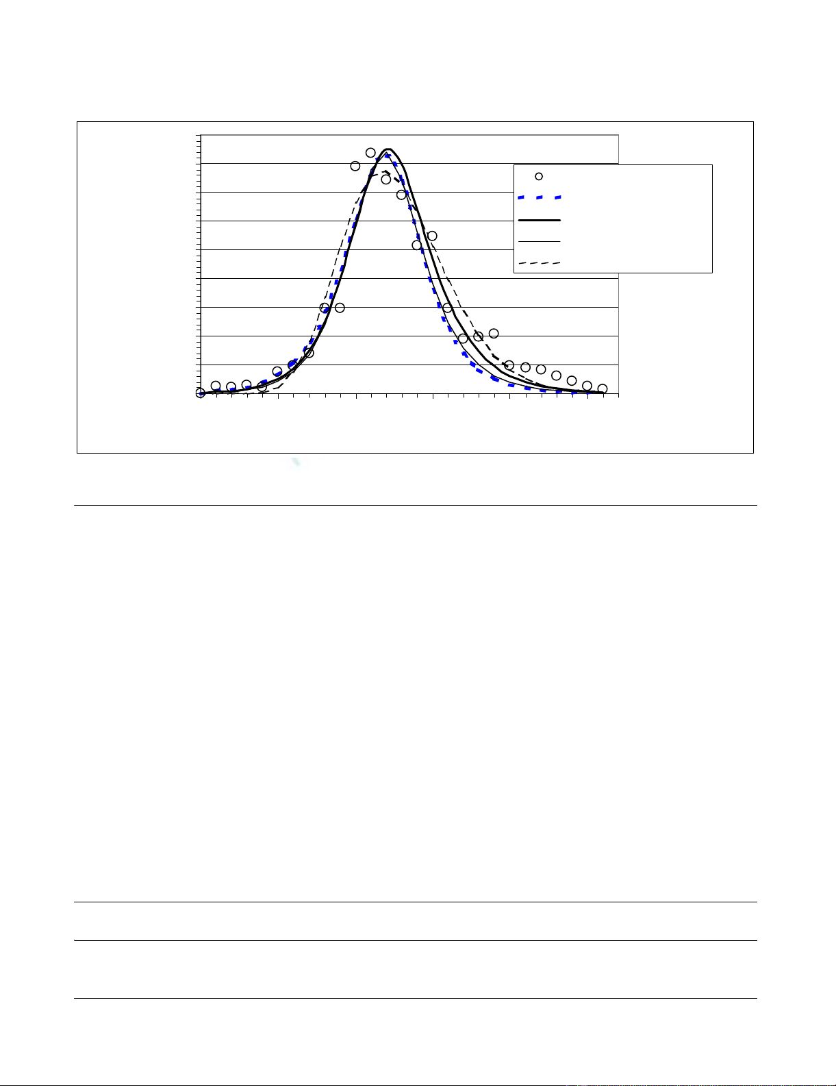
Best-fit incidence curves from the SEIR model for the three
scenarios are shown in Figure 1. The corresponding best-
fit
β
,
ν
and
γ
, and corresponding R0, TE and TI values, are
shown in Table 2. The R0 values ranged between 1.3, and
3.1, and corresponding average latent period and infec-
tious period estimates ranged between 0.7 and 1.3 days,
and 0.2 and 0.3 days, respectively.
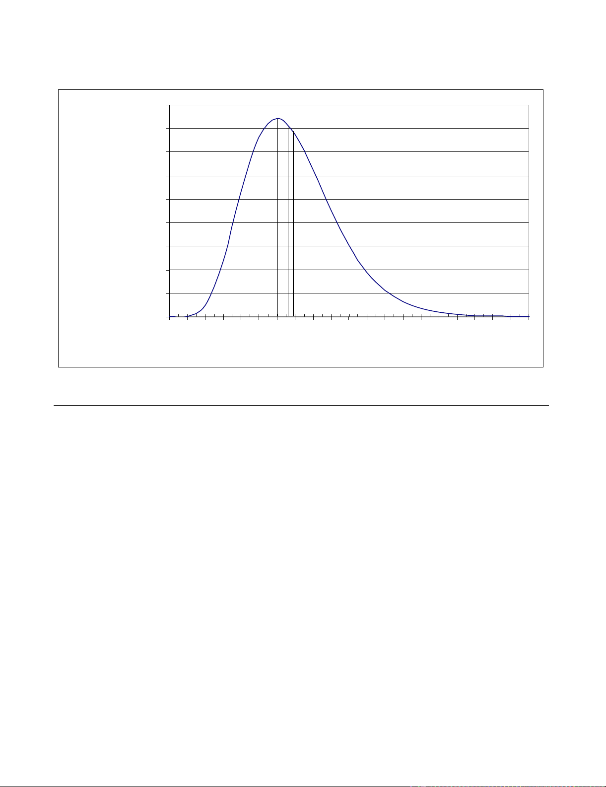
The gamma distribution of incidence-mortality lag time
obtained by convolution is shown in Figure 2. The mean,
median, mode and variance of this distribution are 6.9,
6.6, 6.0 and 6.3 days respectively.
Observed mortality data, shown in Figure 3, indicate
more variability around a best-fit gamma distribution
than observed incidence data (see Figure 1). Mortality
curves for each of Scenarios 1 to 3, obtained by convolu-
tion, all agree well with the best-fit gamma distribution of
observed data.
Discussion
This analysis has demonstrated the potential for using his-
torical disease epidemic data to derive plausible, and
potentially useful, pandemic influenza parameter esti-
mates. This is the first time that these parameters have
been reported for the 1918 pandemic outside of Europe,
the USA and Brazil.
de
dt PPInfsie
ids ids as
=+− −
()
βν
(( ))19
Table 1: Parameters used in the SEIR incidence model*.
Parameter Scenario 1Scenario 2Scenario 3
Initial proportion of the population susceptible (Pis) 1.0 0.9 0.8
Proportion of infected cases who develop symptoms (Pids) 0.95 0.81 0.67
Infectivity of asymptomatic/infectivity of symptomatic people (Infas) 0.6 0.5 0.4
Proportion of symptomatic cases who present and are diagnosed as infected with influenza (Psp) 0.95 0.88 0.8
*Based on plausible ranges for pandemic influenza with Scenario 1 being closer to a worse case for impact on health and Scenario 3 being less
severe. For example, Scenario 3 assumes 20% of the population may have had immunity from previous influenza pandemics that may have reached
New Zealand in the late 19th century – as suggested by Rice [2] and supported by the unusually low mortality rates in the older age groups for this
pandemic in New Zealand [2].
Theoretical Biology and Medical Modelling 2006, 3:38 http://www.tbiomed.com/content/3/1/38
Page 4 of 7
(page number not for citation purposes)
Limitations of this analysis
This work is limited by the very nature of using data from
an event that occurred over eight decades ago. For exam-
ple, the estimate of the camp's population was only
approximate (at 8000). The mortality burden of this par-
ticular outbreak (at 20.4 per 1000) was also somewhat
higher than that for the general male population of New
Zealand (ie, at 10.0 per 1000 for 20–24 year olds) [2]. It
was, however, similar to the pandemic influenza mortal-
ity burden of the armed forces as a whole (at 23.5 per
1000) and for other military camps at 22.0 and 23.5 (for
Awapuni and Trentham camps respectively) [2]. It is plau-
sible that higher death rates in military camps may have
been related to both higher risk of infection (e.g. via
crowding) and the poor living conditions involved (i.e.
the extensive use of tents). Crowded troop trains may also
have contributed to disease spread and in the weekend
prior to the main outbreak in the camp many of the
recruits had been away on leave, and were transported to
and from the camp by troop trains. Furthermore, a severe
storm struck the Featherston camp on 7 November (the
day that influenza incidence peaked) and flattened many
tents. This event placed additional stresses on accommo-
dating men in huts that were already full and with some
huts (and all institute buildings such as the YMCA, for
example) being used as overflow wards to the main camp
hospital to which the most severe cases were admitted.
Less severe cases were admitted to makeshift wards in the
so-called institute buildings, and the huts were used for
convalescence. In his report, the Principal Medical Officer
commented that this storm was likely to have exacerbated
the impact of the outbreak and this is certainly plausible
[3].
In addition to data limitations, the parameters used for
the SEIR model also involve uncertainties; for example,
we have no good data on the proportion of the young
male population who were likely to be susceptible to this
strain in 1918 (e.g. based on the possible residual immu-
nity from the first wave of the pandemic or from previous
Table 2: Rate constants and epidemiological parameters corresponding to the best-fit models shown in Figure 1 (associated standard
deviation or 95% confidence interval is given in brackets).
Scenario
β
(days-1)
ν
(days-1)
γ
(days-1)R0Latent period TE
(days)
Infectious
period TI (days)
1 5.3 (0.50) 1.5 (0.08) 4.2 (0.33) 1.3 (0.02) 0.67 (0.60, 0.74) 0.24 (0.21, 0.28)
2 6.5 (0.27) 1.2 (0.04) 3.6 (0.11) 1.8 (0.04) 0.83 (0.78, 0.89) 0.28 (0.26, 0.30)
3 10.1 (1.55) 0.8 (0.11) 3.3 (0.36) 3.1 (0.18) 1.25 (0.99, 1.69) 0.30 (0.25, 0.38)
Observed and best-fit modelled incidence (ill cases per day) for Scenarios 1 to 3, and best-fit gamma distributionFigure 1
Observed and best-fit modelled incidence (ill cases per day) for Scenarios 1 to 3, and best-fit gamma distribution.
0
50
100
150
200
250
300
350
400
450
0 5 10 15 20 25
Time (days)
Daily
incidence
observed incidence
scenario 1
scenario 2
scenario 3
fitted gamma distribution
Theoretical Biology and Medical Modelling 2006, 3:38 http://www.tbiomed.com/content/3/1/38
Page 5 of 7
(page number not for citation purposes)
influenza epidemics and pandemics). Also, the SEIR
model involves a number of simplifying assumptions,
including a single index case, homogeneous mixing, expo-
nentially distributed residence times in infectious status
categories, and isolation of the military camp.
Estimating R0
The estimates for R0 in the range from 1.3 to 3.1 are the
first such estimates for the 1918 pandemic outside
Europe, the United States and Brazil, so far as we are
aware. However, given the unique aspects of the military
camp (crowded conditions and a young population with
low immunity) it is quite likely that the R0 values esti-
mated in our analysis might tend to over-estimate those
for the general population. Nevertheless, this effect may
have been partly offset by the camp policy of immediate
hospitalisation upon symptoms, effectively reducing
infective contacts.
Our estimated range for R0 is broadly consistent with esti-
mates for this pandemic in the United States (a median R0
of 2.9 for 45 cities) [12]. Other comparable figures for the
1918 pandemic are: 1.7 to 2.0 for the first wave for British
city-level mortality data [13]; 2.0, 1.6 and 1.7 for the first,
second and third waves in the UK respectively [14]; 1.5
and 3.8 in the first and second waves in Geneva respec-
tively [15]; and 2.7 for Sao Paulo in Brazil [16]. The upper
end of our estimated range (R0 = 3.1) may reflect the dif-
ferences between disease transmission in the general pop-
ulation (as per the above cited studies) and transmission
in a crowded military camp with a predominance of
young males.
Considered collectively, these R0 estimates for pandemic
influenza in various countries are not particularly high
when compared to the R0 estimates for various other
infectious diseases [17]. This observation provides some
reassurance that if a strain of influenza with similar viru-
lence were to emerge, then there would be scope for suc-
cessful control measures. Indeed, one model, using R0
values in the 1.1 to 2.4 range, has suggested the possibility
of successful influenza pandemic control [18]. This was
also the case for a model using R0 = 1.8 [19]. Nevertheless,
at the upper end of the estimated range for R0, control
measures may be more difficult, especially if public health
authorities are slow to respond and they have insufficient
access to antivirals and pandemic strain vaccines.
The latent and infectious periods
The average latent and infectious periods were estimated
to be in the range between 0.7 to 1.3 days, and 0.2 to 0.3
days, respectively. The infectious period is short compared
Incidence-mortality lag time distributionFigure 2
Incidence-mortality lag time distribution.
0
0.02
0.04
0.06
0.08
0.1
0.12
0.14
0.16
0.18
0 1 2 3 4 5 6 7 8 9 1011121314151617181920
Lag (days)
Probability
density
mode
median
mean


![Hình ảnh học bệnh não mạch máu nhỏ: Báo cáo [Năm]](https://cdn.tailieu.vn/images/document/thumbnail/2024/20240705/sanhobien01/135x160/1985290001.jpg)