
FEM for Elliptic Problems
Sebastian Gonzalez Pintor
November, 2016
We follow the results from [Joh12] and [And15].
1 Introduction
•Definition of (D), (V) and (M)
•Equivalence (D)⇒(V)⇔(M)
•If u∈ C2then (D)⇐(V)
•Uniqueness of (V).
Outline: Variational form. and Minimization prob.
Lets consider the following two-point boundary value
problem
−u′′(x) = f(x) for x∈(0,1) (D)
u(0) = u(1) = 0
where u′=uxand fis a given continuous function. We
introduce the notation
(u, v) = Z1
0
v(x)w(x) dx
for real valued piecewise continuous bounded functions,
and the linear space
V={v:v∈ C0([0,1]),Z1
0|v′|2dx < ∞,
and v(0) = v(1) = 0}
and the linear functional
F(v) = 1
2(v′, v′)−(f, v).
We can define the problems (M) and (V) as follows:
Find u∈Vsuch that F(u)≤F(v)∀v∈V, (M)
Find u∈Vsuch that (u′, v′) = (f, v)∀v∈V. (V)
Now we will show that if uis a solution of the two-
point boundary value problem (D), then uis a solution
of the variational problem (V) (D⇒V), and that uis
a solution of the variational problem (V) if, and only
if, uis also a solution of the minimization problem (M)
(V⇔M).
Proposition 1 (D⇒V).If u∈ C2is a solution of
the two-point boundary value problem (D), then uis a
solution of the variational problem (V).
Proof. Multiply equation (D) by v∈Vand integrate
over the whole domain
−Z1
0
u′′vdx=Z1
0
fv dx,
then we integrate by parts and use the boundary condi-
tions on the left side to obtain
−Z1
0
u′′vdx=−[u′v]1
0+Z1
0
u′v′dx
=−u′(1)v(1) + u′(0)v(0)
|{z }
v(1)=v(0)=0
+(u′, v′)
= (u′, v′).
We notice that u∈ C2and u(0) = u(1) = 0 implies that
u∈V, and because the choice of v∈Vis arbitrary, the
function usatisfies the equation
(u′, v′) = (f, v)∀v∈V,
what is the same as problem (V).
Proposition 2 (V⇒M).If u∈Vis a solution of
the variational problem (V), then uis a solution of the
minimization problem (M).
Proof. Let us consider an arbitrary function w∈V. We
define v=w−u∈V, so that using the definition of the
functional Fwe have
F(w) = 1
2(w′, w′)−(w, f )
=1
2(v′+u′, v′+u′)−(v+u, f)
=1
2(v′, v′) + (u′, v′) + 1
2(u′, u′)−(v, f)−(u, f)
=1
2(v′, v′) + (u′, v′)−(v, f)
|{z }
(I)
+1
2(u′, u′)−(u, f)
|{z }
(II)
but because uis solution of (V) we have that (I) = 0,
and we can rewrite (II) = F(u), so using that (v′, v′)≥0
we obtain
F(w) = 1
2(v′, v′) + F(u)≥F(u).
Because w∈Vwas chosen arbitrarily, it means that u
is a solution of (M).
Proposition 3 (M⇒V).If u∈Vis a solution of the
minimization problem (M), then uis a solution of the
variational problem (V).
1

Proof. If uis a solution of (M) we have that
F(u)≤F(u+εv),
for all ε∈R, because u+εv ∈Vfor every v∈V. Thus,
the differentiable function
g(ε)≡F(u+εv)
=1
2(u′, u′) + ε(u′, v′) + ε2
2(v′, v′)−(u, f)−ε(v, f)
=1
2(u′, u′)−(u, f) + ε[(u′, v′)−(v, f)] + ε2
2(v′, v′),
has a minimum at ε= 0 and hence g′(0) = 0. But
g′(ε) = (u′, v′)−(v, f) + ε(v′, v′),
and evaluating at ε= 0 we get
g′(0) = (u′, v′)−(v, f) = 0,
hence uis a solution of (V).
We can also show that
Proposition 4 (Uniqueness).A solution to (V)is
uniquely determined.
Proof. Suppose that u1and u2are solutions of (V), i.e.,
u1, u2∈Vand
(u′
1, v′) = (f, v)∀v∈V,
(u′
w, v′) = (f, v)∀v∈V.
Subtracting these two equations and v=u1−u2∈V
gives
Z1
0
(u′
1−u′
2)2dx= 0
which shows that
u′
1(x)−u′
2(x) = 0 ∀x∈[0,1],
so u1−u2is constant in [0,1], which together with the
boundary conditions u1(0) = u2(0) = 0 gives u1(x) =
u2(x), ∀x∈[0,1], and the uniqueness follows.
Also, because every solution of (D) or (M) is also solution
of (V), but the solution of (V) is unique, it follows the
uniqueness of the solutions of (D) and (M). We notice
here that we have not proved yet that the solution exists,
just uniqueness in case of existence. Existence will be
shown later for a general variational problem, given that
it satisfies some conditions.
Last, we show that
Proposition 5. If u′′(x)exists and it is continuous for
a solution of (V), then uis also a solution of (D).
Proof. For this, assuming that uis a solution of (V), we
have
(u′, v′) = (f, v)∀v∈V,
and integrating by parts the first term, using that v(0) =
v(1) = 0 and that u′′ exists we get,
(u′, v′) = (f, v)∀v∈V,
−(u′′, v) = (f, v)∀v∈V,
(f+u′′, v) = 0 ∀v∈V,
but with the assumption that f+u′′ is continuous, this
can only hold if f(x) + u′′(x) = 0 ∀x∈(0,1) .
2 Variational Formulation
•Hilbert Spaces (L2, H1and H1
0)
–Scalar product, Cauchy-Schwarz inequal-
ity and Cauchy sequence
•Natural and Essential boundary conditions
Outline: Hilbert Spaces
Definition 1. A map a(·,·) : V×V→Rthat is sym-
metric and bilinear, i.e., ∀u, v, w ∈V,∀α, β ∈R
a(v, w) = (w, v),(symmetric)
a(αu +βv, w) = αa(u, w) + βa(v, w) (a(·, w)is linear)
a(u, αv +βw) = αa(u, v) + βa(u, w) (a(u, ·)is linear)
is called a scalar product on Vif
a(v, v)>0,∀v∈V, v 6= 0,
and the norm associated with the scalar product is defined
by
||v||a= (a(v, v))1/2,∀v∈V.
Moreover, if <·,·>is a scalar product with correspond-
ing norm || · ||, we have that the following Cauchy-
Schwarz’s inequality is satisfied
|< v, w > | ≤ ||v|| ||w||,∀v, w ∈V.
Definition 2. A linear space Vwith a scalar product
<·,·>and the corresponding norm || · || is said to be
a Hilbert space if Vis complete, i.e., if every Cauchy
sequence with respect to || · || is convergent, where
•a sequence is said to be Cauchy if
∀ε > 0∃N∈Nsuch that ||vi−vj|| < ε if i, j ≥N,
•a sequence is convergent in Vif ∃v∈Vsuch that
∀ε > 0∃N∈Nsuch that ||vi−v|| < ε if i≥N.
Example 2.1. We can see that the space V:=
C0([−1,1]) is a linear space, and that (·,·)V:V×V→R
defined by
(v, w)V=Z1
−1
v(x)w(x) dx,
2
-1 -0.5 0 0.5 1
-0.2
0
0.2
0.4
0.6
0.8
1
1.2
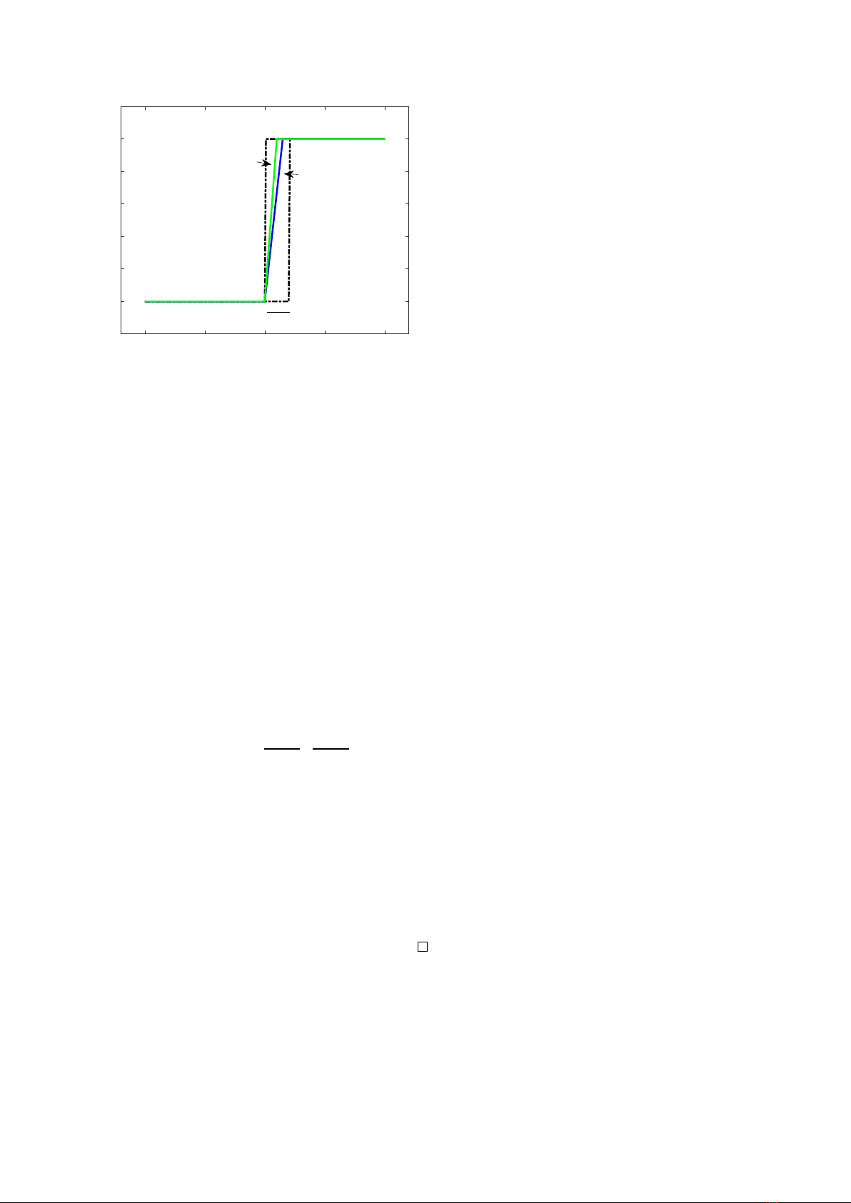
vj
vi
1/N
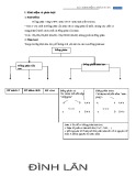
Figure 1: For i, j > N > 1/ε, the square of the area
between viand vjis smaller than ε.
is a scalar product, with the corresponding associated
norm ||v||V= (v, v)1/2
V. But Vwith this norm is not
complete, thus it is not a Hilbert space.
Proof. To see this we can build a Cauchy sequence that
is not convergent inside V. For example, consider the
sequence
vn=
0 if x∈[−1,0],
nx if x∈(0,1/n),
1 if x∈[1/n, 1].
Take ε > 0, and 1/ε < N ∈N, we can see (Figure 1that
the sequence is Cauchy
||vi−vj||2
V=Z1
−1
(vi(x)−vj(x))2dx
=Z1/N
0
0≤·≤1
z}| {
(vi(x)−vj(x))2dx
≤Z1/N
0
dx= 1/N < ε,
but the sequence converges to the function
H(x) = (0 if x∈[−1,0],
1 if x∈(0,1],
which is not inside V. It means that the space Vwith
this norm is not complete, so it is not a Hilbert space.
In particular, for a bounded domain Ω ∈Rd, we define
the following function spaces, with appropriate scalar
products and associated norms, which are Hilbert spaces:
•The linear space of square-integrable functions in a
bounded domain Ω ∈Rd,
L2(Ω) = {v:ZΩ|v|2dx < ∞},
together with the scalar product and its associated
norm as follows
(v, w)L2(Ω) =ZΩ
vw dx,
||v||L2(Ω) =ZΩ
v2dx.
•We also introduce the linear space of square inte-
grable derivatives up to order 1,
H1(Ω) = {v∈L2(Ω), vxi∈L2, i = 1, . . . , d},
together with the scalar product and the associated
norm as follows
(v, w)H1(Ω) =ZΩ
vw +∇v· ∇wdx,
||v||H1(Ω) =ZΩ
v2+|∇v|2dx=||v||L2(Ω) +||∇v||L2(Ω).
•And the space
H1
0(Ω) := {v∈H1(Ω) : v= 0 on Γ},
together with the same scalar product and the as-
sociated norm as for H1(Ω), where Γ := ∂Ω is the
boundary of Ω.
2.1 Boundary Conditions
The boundary conditions for the differential equation are
usually classified as Dirichlet (when they impose a value
for the function on the boundary), Neumann (when they
force a value for the derivative of the function on the
boundary), or mixed (mixing Dirichlet and Newman),
u=gon ∂Ω (Dirichlet)
~n∇u=hon ∂Ω (Neumann)
γu +~n∇u=gon ∂Ω (Mixed)
where g, h, γ are given functions. Building the varia-
tional formulation, when integrating by parts the orig-
inal equation multiplied by a test function, different
boundary conditions will appear in different ways in
the variational formulation. In particular, we focus on
Dirichlet and Neumann boundary conditions, that for
second order differential equations will become essential
and natural boundary conditions, meaning that
•essential boundary conditions will appear in the
function space V, while
•natural boundary conditions will naturally appear
in the variational form.
In general, for an equation of order 2k, the variational
form needs an space with functions differentiable up to
order k, so essential boundary conditions will be inposed
3

in the space for orders 0, . . . , k −1, and natural bound-
ary conditions will be built in the variational form for
orders k, . . . , 2k−1. It is also important to notice that
essential boundary conditions will generate two spaces,
not necessarily the same, one for which the condition is
imposed to the solution, and other one for the test func-
tion where the functions would be zero. For instance,
consider the boundary, Γ, split in two parts, Γ1and Γ2,
then the two spaces are
•u∈V1={v:v∈H1,and v=gon Γ1},
•v∈V2={v:v∈H1,and v= 0 on Γ1},
and they are the same only when g= 0. We notice
that the Neumann boundary conditions do not have any
effect into the function spaces; instead, they will appear
in the variational formulation.
Example 2.2. Consider a bounded domain Ω ∈Rn,
with boundary Γ = ∂Ω∈ C1piecewise, and the bound-
ary is split in two parts Γ1and Γ2. The problem reads
−∆u=fin Ω ⊂Rn,
u=gon Γ1
~n · ∇u=hon Γ2
Proof. We use the spaces
V1={v:v∈H1,and v=gon Γ1},
V2={v:v∈H1,and v= 0 on Γ1},
where the solution must be in V1, and V2is the space of
test functions. Now, multiply the original equation by
a test function vand integrate over the whole domain,
obtaining
−ZΩ
∆uv dx=ZΩ
fv dx, ∀v∈V2,
but integrating by parts (Green’s formula) the left part
−ZΩ
∆uv dx
=ZΩ∇u· ∇vdx−ZΓ
~n∇uv ds
=ZΩ∇u· ∇vdx−ZΓ1
~n∇uv ds
|{z }
v=0 on Γ1
−ZΓ2
~n∇uv ds
|{z }
~n∇u=hon Γ2
=ZΩ∇u· ∇vdx−ZΓ2
hv ds,
so the variational formulation can be rewritten as
Find u∈V1such that
ZΩ∇u· ∇vdx
|{z }
a(u,v)
=ZΩ
fv dx+ZΓ2
hv ds
|{z }
L(v)
,∀v∈V2.
In addition, we can see that the minimization problem
associated to this variational problem can be written by
Find u∈V1such that
F(u)≤F(v)∀v∈V1
where
F(v) = 1
2a(v, v)−L(v),
and it is equivalent to the variational problem above.
3 Existence of solutions:
Lax-Milgram theorem
•Parallelogram law
•Lax-Milgram Theorem
•(V)⇔(M)
•Poincar´e Inequalities for H1and H1
0
•Trace Inequality
Outline: Lax-Milgram
The complete proofs of the following results are provided
in [And15].
Parallelogram Law:Let ||·|| be a norm associated to a
scalar product <·,·>. The following equivalence holds
||x+y||2+||x−y||2= 2||x||2+ 2||y||2.
Theorem 1 (Lax-Milgram).Let Vbe a Hilbert space
with scalar product <·,·>Vand associated norm ||·||V.
Assume that a(·,·)is a bilinear functional and La linear
functional satisfying:
(1) a(·,·)is symmetric, i.e.,
a(v, w) = a(w, v),∀v, w ∈V;
(2) a(·,·)is V-elliptic, i.e.,
∃α > 0s.t. a(v, v)≥α||v||2
V,∀v∈V;
(3) a(·,·)is continuous, i.e.,
∃C∈Rs.t. |a(v, w)| ≤ C||v||V||w||V,∀v, w ∈V;
(4) L(·)is continuous, i.e.,
∃Λ∈Rs.t. |L(v)| ≥ Λ||v||V,∀v∈V;
Then there exists a unique function u∈Vsuch that
a(u, v) = L(v),∀v∈V,
and the following estimate holds
||u||V≤Λ
α.
4

Proof. A sketch of the proof (complete proof in [And15])
•Build a solution of (M): ∃u∈Vsolving (M)
–Norm ||v|| =a(v, v) is equivalent to || · ||V
–We see that β= inf
v∈VF(v)>−∞
–{vi} ⊂ V, with F(vi)→β, is Cauchy.
–Completeness implies that ∃u∈Vs.t. vi→u
–Show that F(u) = β. Thus usolves (M).
•(M)⇒(V): Because of proposition 6.
•Uniqueness: If u1and u2solve (V), subtracting the
equations we obtain a(u1−u2, v) = 0, and using (2)
for v=u1−u2we get the result.
•Estimate: Combining (2) and (4) with (V).
Proposition 6 ((V)⇔(M)).Let aand Lbe such that
they satisfy the conditions of Theorem 1. Then, the fol-
lowing problems are equivalent:
•Find u∈Vsuch that a(u, v) = L(v),∀v∈V; (V)
•Find u∈Vsuch that F(u)≤F(v),∀v∈V; (M)
where F(v) = 1
2a(v, v)−L(v).
Proof. Similar to (V⇔M) before (complete proof
in [And15]).
Example 3.1. Show, using Lax-Milgram theorem, that
the following problem has a unique solution:
Find u∈V:= H1(Ω),Ω⊂R2, such that
ZΩ
(∇u· ∇v+uv) dx=ZΩ
fv dx, ∀v∈H1(Ω)
Proof. Using
a(v, w) := ZΩ
(∇v· ∇w+vw) dx, L(w) := ZΩ
fw dx,
we check for the different conditions:
1. ais clearly symmetric.
2. a(v, v) = ||v||2
H1(Ω) proves V-ellipticity
3. Cauchy-Schwarz in H1(Ω) provides continuity for
|a(v, w)|=||v||H1(Ω)||w||H1(Ω)
4. Cauchy-Schwarz in L2(Ω) provides continuity for
|L(v)|=|(f, v)L2(Ω)|=||f||L2(Ω)||v||L2(Ω) ≤Λ||v||H1(Ω)
with Λ = ||f||L2(Ω).
Thus, using theorem 1there exists a unique solution.
It is sometimes useful to be able to bound the norm of
the function with the bound of the derivative in order to
verify conditions (2) −(4) of the Lax-Milgram theorem.
It is easy to show that this can not be done with constant
functions, so that we can use the followings Poincar´e
inequalities, always having a mechanism that identify
constant functions with the function zero.
Theorem 2 (Poincar´e inequality for H1
0(Ω)).Let Ωbe a
bounded domain in Rnwith boundary ∂Ω∈ C1piecewise.
Let u∈H1
0(Ω). Then there exists a constant C > 0such
that
||u||L2(Ω) ≤C||∇u||L2(Ω).
Proof. A sketch of the proof (complete proof in [And15])
•We use the function φ(x) = 1/(2n)Px2
i, with ∆φ=
1, with the Green’s formula and bcs. to get
||u||2
L2(Ω) =−ZΩ
2u(∇u· ∇φ) dx
•and we use Cauchy-Schwarz inequality and boundness
of φin Ω
−ZΩ
2u(∇u· ∇φ) dx≤C||u||L2(Ω)||∇u||L2(Ω)
Theorem 3 (Poincar´e inequality for H1(Ω)).Let Ωbe a
bounded domain in Rnwith boundary ∂Ω∈ C1piecewise.
Let u∈H1(Ω) and let
¯u=1
|Ω|ZΩ
udx, (¯uis the average over Ω).
Then there exists a constant C > 0such that
||u−¯u||L2(Ω) ≤C||∇u||L2(Ω).
Proof. We skip the proof.
The next result (Trace inequality) can be used to prove
continuity for aor Lwhen boundary integrals are in-
volved, i.e., when Neumann boundary conditions are
used.
Theorem 4 (Trace inequality).Let Ωbe a bounded do-
main in Rnwith boundary ∂Ω∈ C1piecewise. Then
there exists a constant C > 0such that
||u||L2(∂Ω) ≤C||u||1/2
L2(Ω)||u||1/2
H1(Ω).
Proof. We skip the proof.
Example 3.2. Prove, using Lax-Milgram theorem, that
there exists a unique solution for the variational formu-
lation associated to the problem
(−∆u=fin Ω,
u= 0 on ∂Ω.
5


![Bài giảng Giải tích hàm nhiều biến [chuẩn nhất]](https://cdn.tailieu.vn/images/document/thumbnail/2026/20260508/vispacex_27/135x160/91991778472930.jpg)


%20--%3e%3cdefs%3e%3cstyle%3e%20.st0%20{%20fill:%20%23fff;%20}%20.st1%20{%20fill:%20%237800fa;%20}%20%3c/style%3e%3c/defs%3e%3cpath%20class='st1'%20d='M117.78,12.18H43.11c2.9,3.47,4.65,7.94,4.65,12.82,0,5.6-2.3,10.66-6.01,14.29h76.02l7.22-13.56-7.22-13.56Z'/%3e%3cg%3e%3cpath%20class='st0'%20d='M53.58,26.17h-.59v-1.46h.59v-4.96h2.83c1.78,0,2.67.94,2.67,2.82v5.76c0,1.87-.89,2.81-2.67,2.81h-2.83v-4.96ZM55.36,21.37v3.34h1.1v1.46h-1.1v3.34h1.01c.61,0,.91-.37.91-1.1v-5.93c0-.74-.3-1.1-.91-1.1h-1.01Z'/%3e%3cpath%20class='st0'%20d='M65.99,31.14h-1.8l-.31-2.07h-2.19l-.31,2.07h-1.64l1.82-11.39h2.62l1.82,11.39ZM65.28,18.04c-.25.46-.51.77-.75.94-.21.15-.47.22-.79.22-.26,0-.57-.07-.92-.22l-.38-.15c-.14-.05-.26-.07-.37-.07-.3,0-.53.18-.71.54l-.91-.68c.25-.46.51-.77.75-.94.21-.14.48-.21.79-.21.26,0,.57.07.92.21l.38.15c.14.05.26.07.37.07.3,0,.53-.18.71-.54l.91.68ZM61.91,27.52h1.73l-.87-5.76-.87,5.76Z'/%3e%3cpath%20class='st0'%20d='M74.53,26.89v1.52c0,1.91-.89,2.86-2.67,2.86s-2.67-.95-2.67-2.86v-5.93c0-1.91.89-2.86,2.67-2.86s2.67.95,2.67,2.86v1.11h-1.69v-1.22c0-.75-.31-1.12-.93-1.12s-.93.37-.93,1.12v6.15c0,.74.31,1.11.93,1.11s.93-.37.93-1.11v-1.63h1.69Z'/%3e%3cpath%20class='st0'%20d='M81.4,31.14h-1.8l-.31-2.07h-2.19l-.31,2.07h-1.64l1.82-11.39h2.62l1.82,11.39ZM75.9,19.2l1.52-1.91h1.71l1.51,1.91h-1.61l-.76-.95-.75.95h-1.61ZM77.32,27.52h1.73l-.87-5.76-.87,5.76ZM83.1,15.99l-1.76,1.91h-1.26l1.17-1.91h1.86Z'/%3e%3cpath%20class='st0'%20d='M84.86,19.75c1.78,0,2.67.94,2.67,2.82v1.48c0,1.87-.89,2.81-2.67,2.81h-.85v4.28h-1.79v-11.39h2.64ZM84.01,21.37v3.86h.85c.58,0,.87-.36.87-1.08v-1.71c0-.71-.29-1.07-.87-1.07h-.85Z'/%3e%3cpath%20class='st0'%20d='M93.51,19.75c1.78,0,2.67.94,2.67,2.82v1.48c0,1.87-.89,2.81-2.67,2.81h-.85v4.28h-1.79v-11.39h2.64ZM92.66,21.37v3.86h.85c.58,0,.87-.36.87-1.08v-1.71c0-.71-.29-1.07-.87-1.07h-.85Z'/%3e%3cpath%20class='st0'%20d='M98.8,31.14h-1.79v-11.39h1.79v4.88h2.03v-4.88h1.83v11.39h-1.83v-4.88h-2.03v4.88Z'/%3e%3cpath%20class='st0'%20d='M105.36,24.55h2.46v1.62h-2.46v3.34h3.09v1.63h-4.88v-11.39h4.88v1.63h-3.09v3.18ZM108.17,17.29l-1.76,1.91h-1.26l1.17-1.91h1.86Z'/%3e%3cpath%20class='st0'%20d='M112.2,19.75c1.78,0,2.67.94,2.67,2.82v1.48c0,1.87-.89,2.81-2.67,2.81h-.85v4.28h-1.79v-11.39h2.64ZM111.35,21.37v3.86h.85c.58,0,.87-.36.87-1.08v-1.71c0-.71-.29-1.07-.87-1.07h-.85Z'/%3e%3c/g%3e%3ccircle%20class='st1'%20cx='25'%20cy='25'%20r='20'/%3e%3cpath%20class='st0'%20d='M32.78,19.27c2.92,0,4.43,2.55,5.28,5.33l.71,2.17c.14.38-.33.75-.71.75h-5.61c.19-.33.24-.71.09-1.08l-.75-2.45c-.43-1.32-.99-2.64-1.79-3.77.75-.57,1.65-.94,2.78-.94h0ZM25,18.38c3.25,0,4.9,2.78,5.89,5.89l.76,2.45c.14.42-.33.8-.8.8h-11.69c-.42,0-.94-.38-.8-.8l.75-2.45c.99-3.11,2.64-5.89,5.89-5.89h0ZM25,11.35c1.74,0,3.11,1.37,3.11,3.11s-1.37,3.11-3.11,3.11-3.11-1.41-3.11-3.11,1.41-3.11,3.11-3.11h0ZM17.27,19.27c1.08,0,1.98.38,2.73.94-.8,1.13-1.37,2.45-1.74,3.77l-.8,2.45c-.14.38-.05.75.09,1.08h-5.56c-.42,0-.9-.38-.75-.75l.71-2.17c.9-2.78,2.41-5.33,5.33-5.33h0ZM17.27,12.91c1.51,0,2.78,1.27,2.78,2.83s-1.27,2.83-2.78,2.83-2.83-1.27-2.83-2.83,1.27-2.83,2.83-2.83h0ZM32.78,12.91c1.56,0,2.78,1.27,2.78,2.83s-1.23,2.83-2.78,2.83-2.83-1.27-2.83-2.83,1.27-2.83,2.83-2.83h0ZM27.07,28.56v.09c0,.57-.24,1.08-.61,1.46h0v.05c-.38.33-.9.57-1.46.57s-1.08-.24-1.46-.61h0c-.38-.38-.61-.9-.61-1.46v-.09h1.41v.09c0,.19.05.38.19.47v.05c.09.09.28.19.47.19s.38-.09.47-.19v-.05c.14-.09.24-.28.24-.47t-.05-.09h1.41ZM30.99,28.56v.09c0,1.65-.66,3.16-1.74,4.24-1.08,1.08-2.59,1.79-4.24,1.79s-3.16-.71-4.24-1.79l-.05-.05c-1.04-1.08-1.7-2.55-1.7-4.2v-.09h1.41v.09c0,1.27.47,2.4,1.27,3.25h.05c.85.85,1.98,1.37,3.25,1.37s2.4-.52,3.25-1.37c.85-.8,1.37-1.98,1.37-3.25v-.09h1.37ZM34.99,28.56v.09c0,2.78-1.13,5.28-2.92,7.07-1.79,1.79-4.29,2.92-7.07,2.92s-5.23-1.13-7.07-2.92c-1.79-1.79-2.92-4.29-2.92-7.07v-.09h1.41v.09c0,2.4.94,4.53,2.5,6.08,1.56,1.56,3.72,2.5,6.08,2.5s4.52-.94,6.08-2.5c1.56-1.56,2.5-3.68,2.5-6.08v-.09h1.41Z'/%3e%3c/svg%3e)