13
Linear estimation zyxwvutsrqponmlkjihgfedcbaZYXWVUTSRQPONMLKJIHGFEDCBA
13.1. Projections zyxwvutsrqponmlkjihgfedcbaZYXWVUTSRQPONMLKJIHGFEDCBA
..........................
451
13.1.1. zyxwvutsrqponmlkjihgfedcbaZYXWVUTSRQPONMLKJIHGFEDCBA
Linear algebra
........................
451
13.1.2.
Functional analysis
......................
453
13.1.3.
Linear estimation
.......................
454
13.1.4.
Example: derivation
of
the Kalman filter
.........
454
13.2. Conditional expectations
..................
456
13.2.1.
Basics
.............................
456
13.2.2.
Alternative optimality interpretations
...........
457
13.2.3.
Derivation
of
marginal distribution
.............
458
13.2.4.
Example: derivation
of
the Kalman filter
.........
459
13.3. Wiener filters
.........................
460
13.3.1.
Basics
.............................
460
13.3.2.
The non-causal Wiener filter
................
462
13.3.3.
The causal Wiener filter
...................
463
13.3.4.
Wiener signal predictor
...................
464
13.3.5.
An algorithm
.........................
464
13.3.6.
Wiener measurement predictor
...............
466
13.3.7.
The stationary Kalman smoother zyxwvutsrqponmlkjihgfedcbaZYXWVUTSRQPONMLKJIHGFEDCBA
as
a Wiener filter
....
467
13.3.8.
A numerical example
.....................
468
1
3.1.
Projections
The purpose of this section is to get
a
geometric understanding
of
linear es-
timation
.
First. we outline how projections are computed in linear algebra
for finite dimensional vectors
.
Functional analysis generalizes this procedure
to some infinite-dimensional spaces (so-called Hilbert spaces). and finally. we
point out that linear estimation is
a
special case
of
an infinite-dimensional
space
.
As
an example. we derive the Kalman filter
.
13.1
.
1.
linear algebra
The theory presented here can be found in any textbook in linear algebra
.
Suppose that zyxwvutsrqponmlkjihgfedcbaZYXWVUTSRQPONMLKJIHGFEDCBA
X,
y
are two vectors in zyxwvutsrqponmlkjihgfedcbaZYXWVUTSRQPONMLKJIHGFEDCBA
Rm
.
We need the following definitions:
Adaptive Filtering and Change Detection
Fredrik Gustafsson
Copyright © 2000 John Wiley & Sons, Ltd
ISBNs: 0-471-49287-6 (Hardback); 0-470-84161-3 (Electronic)
452
Linear estimation zyxwvutsrqponmlkjihgfedcbaZYXWVUTSRQPONMLKJIHGFEDCBA
0 zyxwvutsrqponmlkjihgfedcbaZYXWVUTSRQPONMLKJIHGFEDCBA
The scalar product is defined by
(X,
y)
=
Czl
xiyi.
The scalar product
is
a
linear operation in data
y.
0
Length is defined by the Euclidean norm
llxll
= zyxwvutsrqponmlkjihgfedcbaZYXWVUTSRQPONMLKJIHGFEDCBA
dm.
0
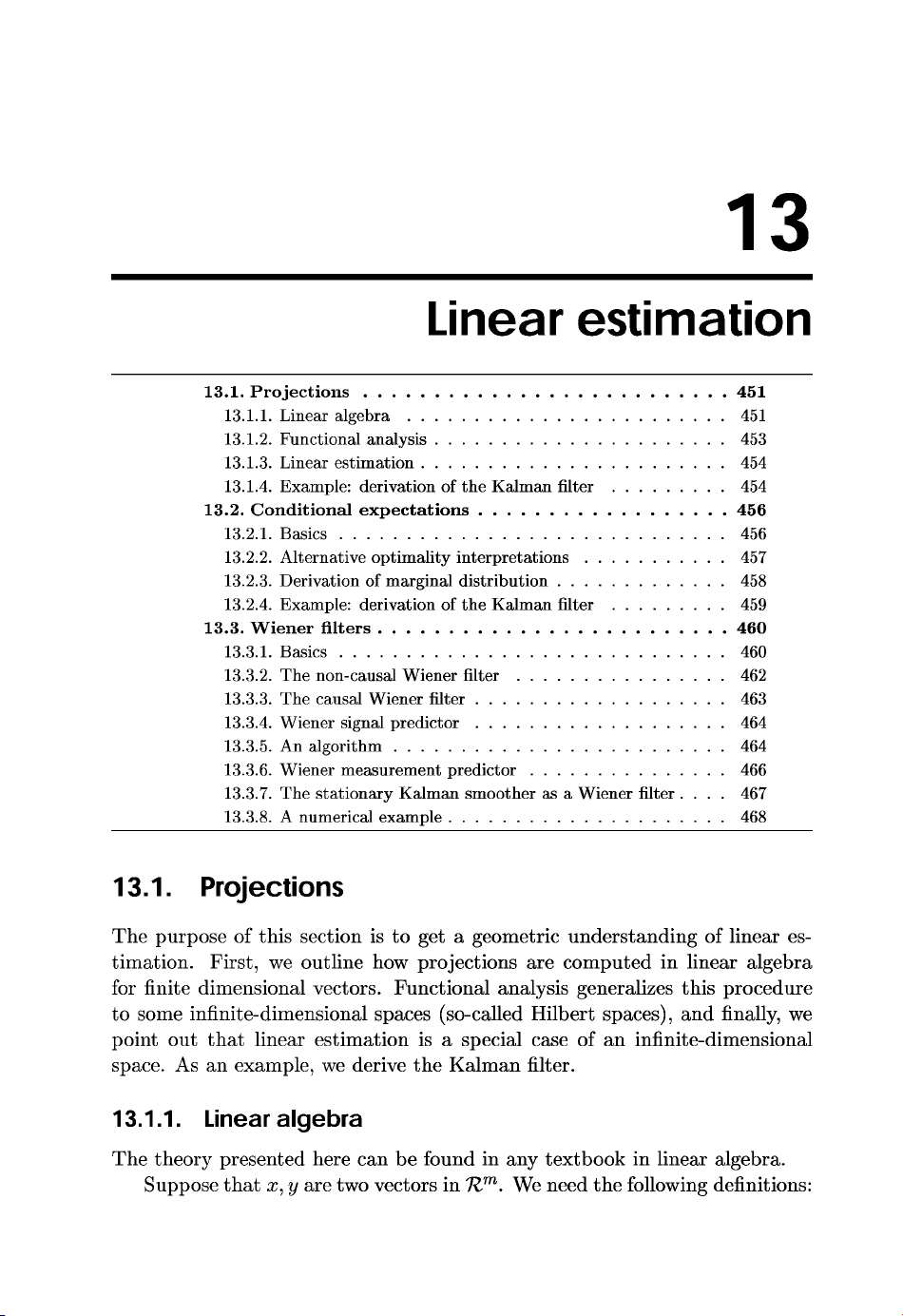
Orthogonality of zyxwvutsrqponmlkjihgfedcbaZYXWVUTSRQPONMLKJIHGFEDCBA
z
and
y
is defined by
(X, y)
=
0:
Ly
0
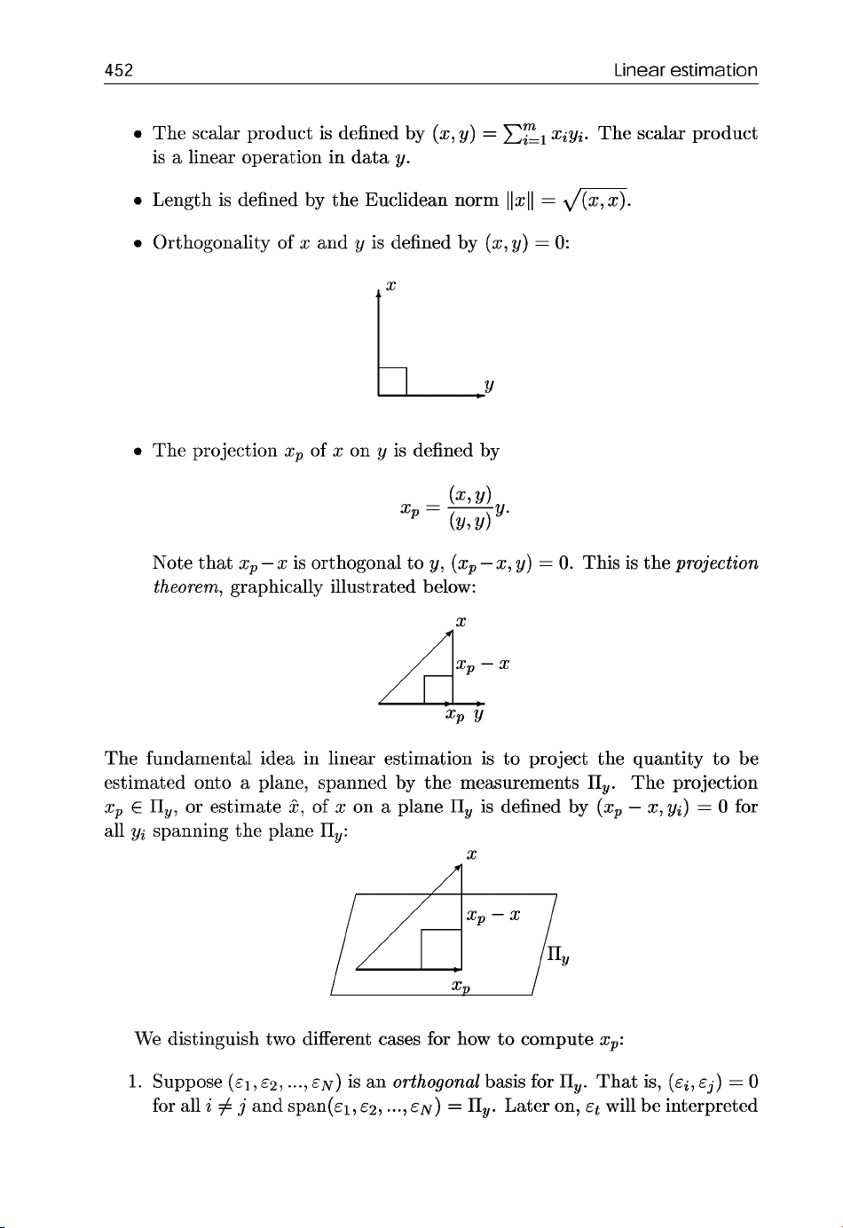
The projection
zp
of
z
on
y
is defined by
Note that
zp zyxwvutsrqponmlkjihgfedcbaZYXWVUTSRQPONMLKJIHGFEDCBA
-X
is orthogonal to
y, (xp
-X,
y)
=
0.
This is the
projection
theorem,
graphically illustrated below:
X
The fundamental idea in linear estimation is to project the quantity to be
estimated onto
a
plane, spanned by the measurements zyxwvutsrqponmlkjihgfedcbaZYXWVUTSRQPONMLKJIHGFEDCBA
IIg.
The projection
zp
E
IIy,
or estimate zyxwvutsrqponmlkjihgfedcbaZYXWVUTSRQPONMLKJIHGFEDCBA
2,
of
z
on
a
plane zyxwvutsrqponmlkjihgfedcbaZYXWVUTSRQPONMLKJIHGFEDCBA
Itg
is defined by
(xP
-
X,
yi)
=
0
for
all
yi
spanning the plane
II,:
X zyxwvutsrqponmlkjihgfedcbaZYXWVUTSRQPONMLKJIHGFEDCBA
I
Xp
I
We distinguish two different cases for how to compute
xp:
1.
Suppose
(~1,
~2,
...,
EN)
is an
orthogonal
basis for
IIg.
That is,
(~i,
~j)
=
0
for all zyxwvutsrqponmlkjihgfedcbaZYXWVUTSRQPONMLKJIHGFEDCBA
i
#
j
and span(e1,
~2,
...,
EN)
=
IIg.
Later on,
Et
will be interpreted
13.1
Proiections
453 zyxwvutsrqponmlkjihgfedcbaZYXWVUTSRQPONMLKJIHGFEDCBA
as the innovations, or prediciton errors. The projection is computed by
Note that the coefficients zyxwvutsrqponmlkjihgfedcbaZYXWVUTSRQPONMLKJIHGFEDCBA
fi
can be interpreted
as a
filter. The projection
theorem
(zP
- zyxwvutsrqponmlkjihgfedcbaZYXWVUTSRQPONMLKJIHGFEDCBA
X, zyxwvutsrqponmlkjihgfedcbaZYXWVUTSRQPONMLKJIHGFEDCBA
~j)
=
0
for all
j
now follows, since zyxwvutsrqponmlkjihgfedcbaZYXWVUTSRQPONMLKJIHGFEDCBA
(xP,
E~)
=
(X,
E~).
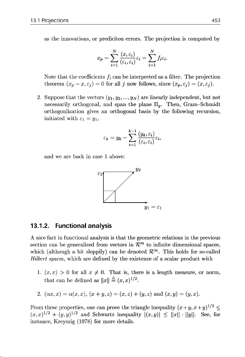
2.
Suppose that the vectors
(yl,
y2,
...,
YN)
are linearly independent, but not
necessarily orthogonal, and span the plane zyxwvutsrqponmlkjihgfedcbaZYXWVUTSRQPONMLKJIHGFEDCBA
IIy.
Then, Gram-Schmidt
orthogonlization gives an orthogonal basis by the following recursion,
initiated with zyxwvutsrqponmlkjihgfedcbaZYXWVUTSRQPONMLKJIHGFEDCBA
€1
=
y1,
and we are back in case
1
above:
Y1
=
E1
13.1.2.
Functional analysis zyxwvutsrqponmlkjihgfedcbaZYXWVUTSRQPONMLKJIHGFEDCBA
A
nice fact in functional analysis is that the geometric relations in the previous
section can be generalized from vectors in
Em
to infinite dimensional spaces,
which (although
a
bit sloppily) can be denoted
Em.
This holds for so-called
Halbert
spaces,
which are defined by the existence of
a
scalar product with
1. zyxwvutsrqponmlkjihgfedcbaZYXWVUTSRQPONMLKJIHGFEDCBA
(z,z)
>
0
for all
IC
#
0.
That is, there is
a
length measure, or norm,
that can be defined
as
llzll
A
(x,x)~/~.
From these properties, one can prove the triangle inequality
(x+Y,
X
+y)lj2
I
(IC,IC)'/~
+
(y,y)II2
and Schwartz inequality
I(x,y)l
5
llzll
.
Ilyll.
See, for
instance, Kreyszig
(1978)
for more details.
454
Linear estimation zyxwvutsrqponmlkjihgfedcbaZYXWVUTSRQPONMLKJIHGFEDCBA
13.1.3. linear estimation zyxwvutsrqponmlkjihgfedcbaZYXWVUTSRQPONMLKJIHGFEDCBA
In linear estimation, the elements
z
and
y
are stochastic variables, or vectors
of stochastic variables.
It
can easily be checked that the covariance defines
a
scalar product (here assuming zero mean),
which satisfies the three postulates for
a
Hilbert space. zyxwvutsrqponmlkjihgfedcbaZYXWVUTSRQPONMLKJIHGFEDCBA
A
linear filter that is optimal in the sense of minimizing the 2-norm implied
by the scalar product, can be recursively implemented as
a
recursive Gram-
Schmidt orthogonalization and
a
projection. For scalar
y
and vector valued
z,
the recursion becomes
Remarks: zyxwvutsrqponmlkjihgfedcbaZYXWVUTSRQPONMLKJIHGFEDCBA
0
This is not
a
recursive algorithm in the sense that the number of com-
putations and memory is limited in each time step. Further application-
specific simplifications are needed to achieve this.
0
To
get expressions for the expectations,
a
signal model is needed. Basi-
cally, this model is the only difference between different algorithms.
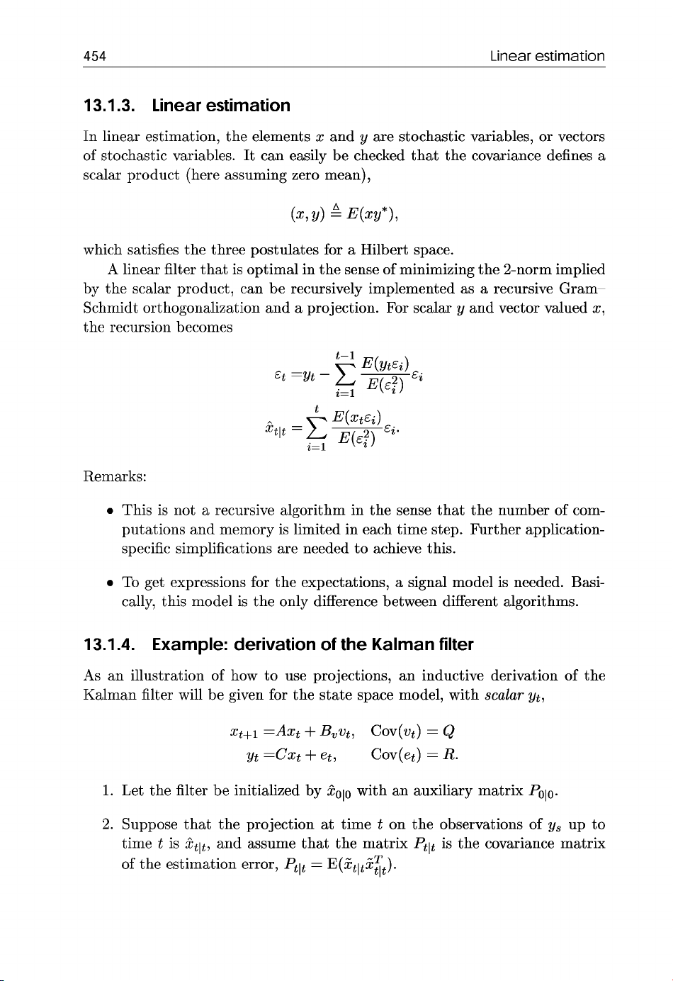
13.1.4. Example: derivation
of
the Kalman filter
As
an illustration of how to use projections, an inductive derivation of the
Kalman filter will be given for the state space model, with zyxwvutsrqponmlkjihgfedcbaZYXWVUTSRQPONMLKJIHGFEDCBA
scalar
yt,
1.
Let the filter be initialized by
iolo
with an auxiliary matrix
Polo.
2.
Suppose that the projection at time
t
on the observations of
ys
up to
time
t
is
Ztlt,
and assume that the matrix
Ptlt
is the covariance matrix
of
the estimation error,
Ptlt
=
E(ZtltZ&).
13.1
Proiections
455 zyxwvutsrqponmlkjihgfedcbaZYXWVUTSRQPONMLKJIHGFEDCBA
3. zyxwvutsrqponmlkjihgfedcbaZYXWVUTSRQPONMLKJIHGFEDCBA
Time update.
Define the linear projection operator by
Then
=AProj(stIyt)
+
Proj(B,vtIyt)
= zyxwvutsrqponmlkjihgfedcbaZYXWVUTSRQPONMLKJIHGFEDCBA
A2+.
-
=O
Define the estimation error as
which gives
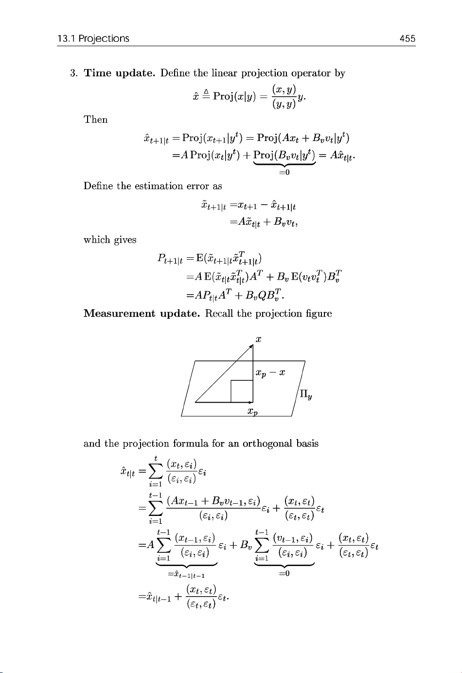
Measurement update.
Recall the projection figure
X zyxwvutsrqponmlkjihgfedcbaZYXWVUTSRQPONMLKJIHGFEDCBA
I
Xp
I
and the projection formula for an orthogonal basis