Báo cáo hóa học: " Properties of Orthogonal Gaussian-Hermite Moments and Their Applications"

Chia sẻ: Linh Ha | Ngày: | Loại File: PDF | Số trang:12

Thêm vào BST

Báo xấu

47
lượt xem 4
download

Download Vui lòng tải xuống để xem tài liệu đầy đủ

Tuyển tập báo cáo các nghiên cứu khoa học quốc tế ngành hóa học dành cho các bạn yêu hóa học tham khảo đề tài: Properties of Orthogonal Gaussian-Hermite Moments and Their Applications

Chủ đề:

Bình luận(0) Đăng nhập để gửi bình luận!

Lưu

Nội dung Text: Báo cáo hóa học: " Properties of Orthogonal Gaussian-Hermite Moments and Their Applications"

EURASIP Journal on Applied Signal Processing 2005:4, 588–599 c 2005 Hindawi Publishing Corporation Properties of Orthogonal Gaussian-Hermite Moments and Their Applications Youfu Wu EGID Institut, Universit´ Michele de Montaigne Bordeaux 3, 1 All´e Daguin, Domaine Universitaire, 33607 Pessac Cedex, France e e Email: youfu wu 64@yahoo.com.cn Jun Shen EGID Institut, Universit´ Michele de Montaigne Bordeaux 3, 1 All´e Daguin, Domaine Universitaire, 33607 Pessac Cedex, France e e Received 7 May 2004; Revised 5 September 2004; Recommended for Publication by Moon Gi Kang Moments are widely used in pattern recognition, image processing, and computer vision and multiresolution analysis. In this paper, we ﬁrst point out some properties of the orthogonal Gaussian-Hermite moments, and propose a new method to detect the moving objects by using the orthogonal Gaussian-Hermite moments. The experiment results are reported, which show the good performance of our method. Keywords and phrases: orthogonal Gaussian-Hermite moments, detecting moving objects, object segmentation, Gaussian ﬁlter, localization errors. 1. INTRODUCTION objects in a visible range of the video camera [2, 11, 12, 13, 14, 15, 16, 17, 18, 19, 20, 21, 22]. The objects can be persons, vehicles, animals, etc. [2, 12, 13, 15, 21, 23, 24]. Moments are widely used in pattern recognition, image pro- In general, we can classify the methods of detecting the cessing, and computer vision and multiresolution analysis moving objects in an image sequence into three principal [1, 2, 3, 4, 5, 6, 7, 8, 9]. We present in this paper a study on or- categories: methods based on the background subtraction thogonal Gaussian-Hermite moments (OGHMs), their cal- (BS) [2, 12, 13, 18], methods based on the temporal varia- culation, properties, application and so forth. We at ﬁrst an- tion in the successive images [1, 2, 25], and methods based alyze their properties in spatial domain. Our analysis shows orthogonal moment’s base functions of diﬀerent orders hav- on stochastic estimation of activities [11]. ing diﬀerent number of zero crossings and very diﬀerent To extract the background image, one simple method is to take the temporal average of the image sequence; another shapes, therefore they can better separate image features based on diﬀerent modes, which is very interesting for pat- is to take the median of the image sequence [2]. However, these methods are likely to be ineﬀective to solve the prob- tern analysis, shape classiﬁcation, and detection of the mov- lems of the lighting condition change between the frames ing objects. Moreover, the base functions of OGHMs are and the slow moving objects. For example, the mean method much more smoothed; are thus less sensitive to noise and leaves the trail of the slow moving object in the background avoid the artefacts introduced by window function’s discon- image, which may lead to the wrong detecting results. tinuity [1, 5, 10]. In order to obtain the background image almost on real Since the Gaussian-Hermite moments are much time, the adaptive background subtraction (ABS) method, smoother than other moments [5], and much less sensitive proposed by Stauﬀer and Grimson [12, 13], can be adopted. to noise, OGHMs could facilitate the detection of moving In this method, a mixture of K Gaussian distributions objects in noisy image sequences. Compared with other diﬀerential methods (DMs), experiments show that much adaptively models each pixel of intensity. The distributions are evaluated to determine which are more likely to re- better results can be obtained by using the OGHMs for the sult from a background process. This method can deal moving objects detection. Traﬃc management and information systems rely on with the long-term change in lighting conditions and scene some sensors for estimating traﬃc parameters. Vision-based changes. However, it cannot deal with sudden movements video monitoring systems oﬀer a number of advantages. The of the uninteresting objects, such as the ﬂag waving or winds blowing through trees for a short burst of time [11]. ﬁrst task for automatic surveillance is to detect the moving
Orthogonal Moments and Their Applications 589 A sudden lighting change will then cause the complete frame In particular, to be regarded as foreground, if such a condition arises. The algorithm needs to be reinitialized [11, 12, 13]. It again de- M0 x, s(x) = g (x, σ ) ∗ s(x), mands a certain quantity of accumulated images. (6) d Our paper is organized as follows. Section 2 presents M1 x, s(x) = 2σ g (x, σ ) ∗ s(x), OGHMs and their properties; Section 3 presents the detec- dx tion of the moving objects by using OGHMs; Section 4 gives the experimental results and the performance comparison where “∗” represents the operation of convolution. with other methods of detecting the moving objects; some In the 2D case, the OGHMs of order ( p, q) of an input conclusions and discussions are presented in Section 5. image I (x, y ) can be deﬁned similarly as M p , q x , y , I (x , y ) 2. OGHMS AND THEIR PROPERTIES ∝ ∝ uv 2.1. Hermite moments [5, 6] = g (u, v, σ )H p,q I (x + u, y + v)dudv , , σσ −∝ ∝ Hermite polynomial is one family of the orthogonal polyno- (7) mials as follows: where H p,q (u/σ , v/σ ) = H p (u/σ )Hq (v/σ ), g (u, v, σ ) = (1/ t Pn = Hn , (1) 2πσ 2 ) exp(−(u2 / 2σ 2 + v2 / 2σ 2 )). σ Obviously, the 2D OGHMs are separable, so the calcula- where Hn (t ) = (−1)n exp(t 2 )(dn /dt n ) exp(−t 2 ), σ is the stan- tion of the 2D OGHMs can be decomposed into the cascade of two steps of the 1D OGHMs calculation: dard deviation of the Gaussian function. The 1D nth-order Hermite moment Mn (x, s(x)) of a sig- nal s(s) can therefore be deﬁned as follows: M p , q x , y , I (x , y ) ∝ ∝ ∝ u = Mn x, s(x) = g (u, δ )H p I (x + u, y + v)du s(x + t )Pn (t )dt (8) σ −∝ ∝ −∝ (2) = Pn (t ), s(x + t ) (n = 0, 1, 2, . . . ). v × g (v , σ )H p dv. σ In the 2D case, the 2D ( p, q)-order Hermite moment is In order to detect moving objects in image sequences by deﬁned as using OGHMs, if a video image sequence { f (x, y , t )}t=0,1,2,... M p , q x , y , I (x , y ) is given, for each spatial position (x, y ) on the images, we deﬁne the temporal OGHMs as follows: (3) ∝ ∝ uv = I (x + u, y + v)H p,q dudv, , σσ −∝ ∝ ∝ Mn t , f ( x , y , t ) = f (x, y , t + v)Bn (v)dv. (9) where I (x, y ) is an image and H p,q (u/σ , v/δ ) = H p (u/σ ) × −∝ Hq (v/σ ). Its recursive algorithm can be rewritten as follows: 2.2. Orthogonal Gaussian-Hermite moments Mn t , f (x, y , t ) The OGHMs was proposed by Shen et al. [5, 6]. The OGHMs = 2(n − 1)Mn−2 t , f (x, y , t ) + 2σMn−1 t , f (1) (x, y , t ) . of a signal s(x) is deﬁned as (10) ∝ Mn x, s(x) = s(x + t )Bn (t )dt = Bn (t ), s(x + t ) , (4) In particular, we use only the moments of the odd orders −∝ up to 5. √ where Bn (t ) = g (t , σ )Pn (t ), g (x, σ ) = (1/ 2πσ ) exp(−x2 / 2σ 2 ) and Pn (t ) is a Hermite polynomial function. 2.3. The properties of the OGHMs For calculating the OGHMs, we can use the following re- First of all, the Gaussian ﬁlter has a property as follows: cursive algorithm: dn Mn x, s(m) (x) = 2(n − 1)Mn−2 x, s(m) (x) g (t , σ ) ∗ f (x, y , t ) = g (n) (t , σ ) ∗ f (x, y , t ). (11) dt n (5) + 2σMn−1 x, s(m+1) (x) (n ≥ 2), According to the recursive algorithm, the OGHMs have where s(m) (x) = (dm /dxm )s(x), s(0) (x) = s(x). the following properties.
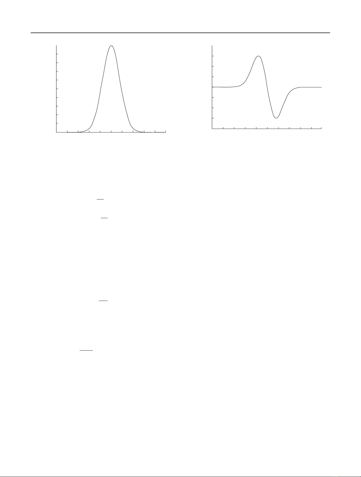
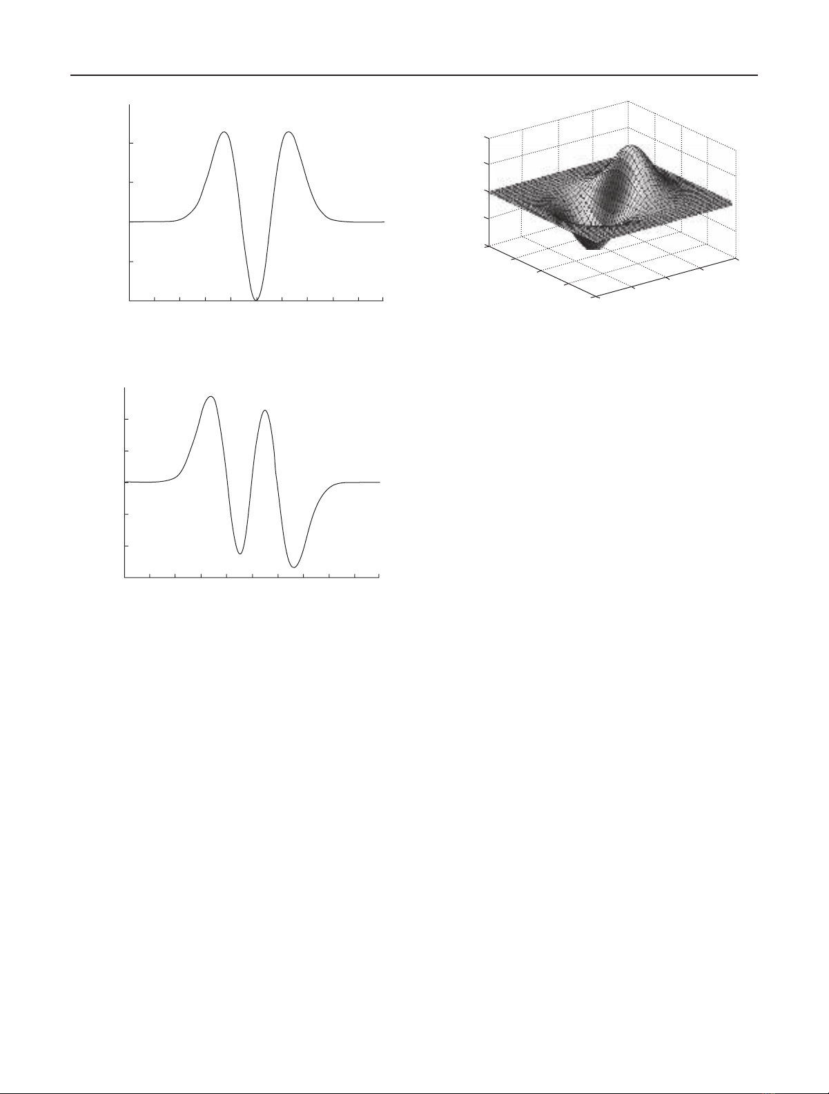
590 EURASIP Journal on Applied Signal Processing 0.5 0.8 0.45 0.6 (−2 ∗ x/σ ) ∗ g (x, σ ), σ = 0.8 0.4 0.4 0.35 g (x, σ ), σ = 0.8 0.2 0.3 0 0.25 −0.2 0.2 0.15 −0.4 0.1 −0.6 0.05 −0.8 −5 −4 −3 −2 −1 0 0 1 2 3 4 5 −5 −4 −3 −2 −1 0 1 2 3 4 5 x x Figure 2: The mask of the 1D OGHMs of order 1. Figure 1: The mask of the 1D OGHMs of order 0. dt i )(g (t , σ ) ∗ f (x, y , t )), we note that F (t , δ ) = n=0 ai (di / Property 1. Given a Gaussian function g (t , σ ) and an image i dt i )g (t , σ ); then F (t , σ ) = 0 has n diﬀerent real roots in the f (x, y , t ) of the image sequence { f (x, y , t )}t=0,1,2,... , we have interval (−∞, ∞). n di Mn t , f ( x , y , t ) = g (t , σ ) ∗ f (x , y , t ) ai F (x, σ ) is called the base function of the OGHMs (also dt i i=0 called the mask of the OGHMs). This property shows that (12) n di the mask of the nth moment has n diﬀerent zero crossings. = g (t , σ ) ∗ f (x, y , t ), ai dt i i=0 2.4. Some conclusions where ai depends on σ only. From the properties of OGHMs, we see that these moments are in fact linear combinations of the derivatives of the ﬁl- n i i i=0 ai (d /dt )g (t , σ ) This property shows that the mask tered signal by a Gaussian ﬁlter. As it is well known, deriva- of the nth moment is the linear combination of the Gaussian tives are important features widely used in signal and im- function and its derivatives of diﬀerent orders. age processing. Because diﬀerential operations are sensitive to random noise, a smoothing is in general necessary. The Property 2. Given a Gaussian function g (t , σ ) and an image Gaussian-Hermite moments just meet this demand because sequence { f (x, y , t )}t=0,1,2,... , we have of the Gaussian smoothing included. In image processing, one often needs the derivatives of diﬀerent orders to eﬀec- k d 2i tively characterize the images, but how to combine them is Mn t , f ( x , y , t ) = g (t , σ ) ∗ f (x , y , t ) a2i dt 2i still a diﬃcult problem. The OGHMs show a way to construct (13) i=0 orthogonal features from diﬀerent derivatives. for n = 2k (n is even), For facilely understanding the OGHMs, in Figures 1, 2, 3, 4, and 5, we give out some characteristics charts of the base function of OGHMs. Mn t , f ( x , y , t ) In the spatial domain, because the base function of the k d2i+1 nth-order OGHMs will change its sign n times, OGHMs can = g (t , σ ) ∗ f (x , y , t ) , (14) a2i+1 well characterize diﬀerent spatial modes as other orthogonal dt 2i+1 i=0 moments. As to the frequency domain behavior, because the for n = 2k + 1 (n is odd), base function of the nth-order OGHMs consists of more os- cillations when the order n is increased, they will thus contain where ai depends on σ only. more and more frequency. Table 1 shows that the frequency windows’ quality factor Q = (center/eﬀective bandwidth) of This property shows that the mask of the OGHMs of odd OGHMs base function is large than that of other moment order is the linear combination of the derivatives of odd or- base function; therefore OGHMs separate diﬀerent bands ders of the Gaussian function, and the mask of the OGHMs more eﬃciently. Moreover, from the properties of OGHMs, of even order is the linear combination of the derivatives of we see that these moments are in fact linear combinations even orders of the Gaussian function. of the derivatives of the signal ﬁltered by a Gaussian ﬁlter, therefore, realizing diﬀerential operation and removing ran- Property 3. Given a Gaussian function g (t , σ ) and an image sequence { f (x, y , t )}t=0,1,2,... , Mn (t , f (x, y , t )) = n=0 ai (di / dom noise. i
Orthogonal Moments and Their Applications 591 1.5 0.1 (−x/σ )g (x, y , σ ), σ = 0.8 1 2nd (F (x, σ ), σ = 0.8) 0.05 0.5 0 −0.05 0 −0.1 2 −0.5 1 2 0 1 y 0 −1 −1 −1 −2 −2 x −5 −4 −3 −2 −1 0 1 2 3 4 5 x Figure 5: The mask of the 2D OGHMs of order (1, 0). Figure 3: The mask of the 1D OGHMs of order 2. 3 are much smoother than other moments, therefore much less sensitive to noise, which could facilitate the detection of the 2 moving objects in noisy image sequences. To detect the moving objects by using the OGHMs, we 3rd (F (x, σ ), σ = 0.8) 1 ﬁrst calculate the temporal moments of an image sequence. According to (14), calculating the temporal OGHMs of an 0 image sequence is equal to calculating the convolution of the mask F (t , σ ) with f (x, y , t ). In order to approach the mask F (t , σ ), according to the inequality |t−Et|≥ε g (t )dt ≤ −1 (1/ε2 ) (t − Et )2 g (t )dt = σ 2 /ε2 , if we take ε = 5σ , then |t −Et |≥ε g (t )dt ≤ 1/ 25 = 4%. Hence the Gaussian function as −2 the convolution kernel is common to choose No = 10σ + 1, −3 namely the masks of size 2L + 1 with L = 5σ is used. For −5 −4 −3 −2 −1 0 1 2 3 4 5 practical computation reasons, we use only the moments of x orders up to 5. Hence, in order to detect the moving objects using the OGHMs, the temporal OGHMs of an image se- Figure 4: The mask of the 1D OGHMs of order 3. quence is calculated ﬁrst. Since both the positive values and negative values of the From the viewpoint of frequency analysis, it seems that moments correspond to the moving objects (containing the the OGHMs characterize images more eﬃciently. With the noise), we take the absolute value of the moments instead of help of the technique representing frequency characteristics their original values. For example, for Figure 6, from Figure 7 by the band center ω0 and eﬀective bandwidth Be , we can bet- to Figure 11, we present the OGHMs images, visualized by ter see the diﬀerences between the moment base functions. linearly transforming the absolute value of the OGHMs to In Table 1, these characteristics for orders from 0 through 10 the gray value ranging from 0 to 255. It can be seen that four are shown. A similar conclusion holds in 2D cases. In general, moving objects (2 persons, one car, and one cyclist) are well one uses the max order up to 10. enhanced in the moment images. Thus M3 contains more information than M1 for de- tecting the moving objects. Therefore, we can use the third 3. DETECTING MOVING OBJECTS USING OGHMS moment to detect the mobile objects. Figures 8 and 9 show 3.1. Calculating the OGHMs images the experimental results in this case. By comparing the results obtained in the case of σ = 0.3 According to (12), (13), and (14), we can see that all the OGHMs are actually the linear combinations of the diﬀerent and σ = 0.8, it can be seen when a larger σ is used, the results of the detection of the moving objects are less sensitive to the order derivatives of the image ﬁltered by a temporal Gaus- noises, but the detected objects have larger sizes than their sian ﬁlter. As it is well known, the temporal derivatives can real sizes. This phenomenon can be explained in Section 3.4. be used to detect the moving objects in image sequences. The The M5 is a weighted sum of the ﬁrst-, third-, and ﬁfth- OGHMs of odd orders are in fact the combinations of these order derivatives of image ﬁltered by a temporal Gaussian ﬁl- derivatives, it is therefore reasonable to use them to detect the ter. Therefore, M5 still contains more information than these moving objects. M1 and M3 for the detection of the moving objects. Figures According to (12), Mn is equal to the temporal derivative 10 and 11 show the experiment results. of the image ﬁltered by a Gaussian ﬁlter, and the OGHMs
592 EURASIP Journal on Applied Signal Processing Table 1: Frequency characteristics of the base functions of geometric, Hermite, Legendre moments, and OGHMs. Moment Geometric moment Hermite moment Legendre moment OGHMs ω0 Be ω0 /Be ω0 Be ω0 /Be ω0 Be ω0 /Be ω0 Be ω0 /Be order 0 0.40 2.11 0.1896 0.40 2.11 0.1896 0.40 2.11 0.1896 0.53 0.44 1.2045 1 1.25 3.87 0.3230 1.25 3.87 0.3230 1.25 3.87 0.3230 1.13 0.48 2.3542 2 1.59 4.71 0.3376 1.64 4.77 0.3438 1.94 4.90 0.3959 1.36 0.75 1.8133 3 2.32 5.74 0.4042 2.42 5.86 0.4130 2.60 5.74 0.4530 1.69 0.80 2.1125 4 2.61 6.23 0.4189 2.79 6.45 0.4326 3.25 6.46 0.5031 1.86 0.97 1.9175 5 3.28 7.00 0.4686 3.56 7.30 0.4877 3.92 7.15 0.5483 2.12 1.01 2.0990 6 3.52 7.36 0.4783 3.93 7.78 0.5051 4.59 7.77 0.5907 2.24 1.15 1.9478 7 4.15 7.98 0.5201 4.69 8.50 0.5518 5.29 8.41 0.6290 2.47 1.19 2.0756 8 4.36 8.27 0.5272 5.10 8.94 0.5705 6.01 9.01 0.6670 2.59 1.33 1.9474 9 4.95 8.79 0.5631 5.89 9.59 0.6142 6.77 9.64 0.7023 2.81 1.41 1.9929 10 5.14 9.03 0.5692 6.36 10.03 0.6341 7.55 10.23 0.7380 2.97 1.66 1.7892 3.2. Detecting the moving objects by integrating function [2]: the ﬁrst, third, and ﬁfth moments π M (x, y ); T , Mmin (x, y ) It is known that the third and ﬁfth moments contain more   2 2 T − M (x , y )  information than the ﬁrst moment, so we can integrate the  1 −    ﬁrst, third, and ﬁfth moments. 2  T − Mmin (x, y )     Because the ﬁrst, third, and ﬁfth moments are orthogo-   T − M (x , y )   nal, one can consider that the ﬁrst moment is the projection  ≤ 0.5, if 0 <   T − Mmin (x, y )   of image f (x, y , t ) on axis 1; the third moment is the pro-      jection of image f (x, y , t ) on axis 3; the ﬁfth moment is the 2  T − M (x , y )  (15) −1 2 projection of image f (x, y , t ) on axis 5; and the axes 1, 3, = T − Mmin (x, y )   and 5 are orthogonal. For getting the perfect real moving ob-     T − M (x , y )  jects using the ﬁrst, third, and ﬁfth moments, we may use the   ≤ 1, if 0.5 <   vector module of the 3D space to regain its actual measure,  T − Mmin (x, y )      2 2 2 namely M (x, y , t ) = M1 + M3 + M5 .   1 if M (x, y ) ≥ T ,   Henceforward, we principally adopt the M (x, y , t ) as      OGHMs images (OGHMIs). We notice that the OGHMIs  0 otherwise, contain more information than a single derivative image or single OGHMs. where M (x, y ) is the gray level of the OGHMI at the point (x, y ), T is the segmentation threshold of the 3.3. Segmenting the motion objects moment image M (x, y ), which is obtained by using the (IMM) [2], Mmin (x, y ) is the minimum of M (x, y ). We have noticed that OGHMI (OGHM) is also equal to the π (M (x, y ); T , Mmin (x, y )) is still noted as π (x, y ). image transformation. This transformation can suppress the For each point in the moment images, the membership background, and enhance the motion information. We also function, which gives a measure of the “mobility” of each know, for the noise image, we cannot remove all noise by pixel in each moment image, is ﬁrst determined. We then a Gaussian ﬁlter. For obtaining the true region of the mov- apply a fuzzy relaxation to the membership function im- ing objects, having calculated the OGHMIs, we then detect ages, which gives the ﬁnal results of the moving pixel detec- the moving objects by the use of the segmentation of such tion [2]. images. To do this, a threshold for each OGHMI should be determined. One of the well-known methods for the 3.4. Analyzing the localization errors threshold determination for image segmentation is the in- variable moments method (IMM) [2, 3, 25]. But this method According to the theory of Gaussian ﬁltering, a Gaussian has not taken into account the spatial and temporal rela- ﬁlter with larger standard deviation is less sensitive to the tions between moving pixels, which are important for im- noises, but brings larger localization errors [26]. How much age sequence analysis. To improve the method, instead of us- is the localization error of detecting the moving objects? Now ing a binary segmentation based on the threshold thus de- we give the discussion. Let F (x, y , t ) = ( f (x, y , t ) + n(x, y , t )) be the input image; termined, we use a fuzzy relaxation for the segmentation of the moment images by taking into account these rela- n(x, y , t ) is the Gaussian white noise image; f (x, y , t ) is the tions with the help of a nonsymmetric π fuzzy membership true image at time t . Given the image F (x, y , t ), the Gaussian
Orthogonal Moments and Their Applications 593 Figure 9: Third OGHMs image (σ = 0.8). Figure 6: Initial image. Figure 10: Fifth OGHMs image (σ = 0.3). Figure 7: First OGHMs image. Figure 8: Third OGHMs image (σ = 0.3). Figure 11: Fifth OGHMs image (σ = 0.8). Supposing the noise variance is n2 (x, y ), then the noise ﬁlter (ﬁnite impulse response) output is as follows: 0 output satisﬁes HF x, y , t0 = f (x, y , t ) ∗ g (t ) + n(x, y , t ) ∗ g (t ), (16) 1/ 2 w 2 1/ 2 g 2 (t )dt E Hn = E n(x, y , t ) ∗ g (t ) = n0 , so we have −w (18) w H f (x, y , 0) = f (x, y , t ) ∗ g (t ) = f (x, y , −t )g (t )dt, −w where H f (x, y , t ) and Hn (x, y , t ) are ﬁlter responses to im- (17) age and noise, respectively. Let true edge point (we consider where ω is the length of integrating windows; in general, ω = that the boundary of the background and the moving object 5σ . point belong to the step-type edge, so its second derivative is
594 EURASIP Journal on Applied Signal Processing zero at the edge point [27]) at t = 0; and let t0 be the edge point of the total response HF (x, y , t ) (in fact, localization er- ror point). Then, HF x, y , t0 = H f x, y , t0 + Hn x, y , t0 = 0, (19) where “ ” represents the derivative of a function on t . Taylor expansion of H f (x, y , t0 ) at t = 0 is as follows: 2 H f x, y , t0 = H f (x, y , 0) + t0 H f (x, y , 0) + O t0 , (20) where H f (x, y , 0) = 0 is assumed (the true edge point). We ignore the higher-order terms. Combining (19) and (20), we have Figure 12: Initial image 0975. t0 H f (x, y , 0) ≈ −Hn x, y , t0 . (21) From a derivative similar to that for noise, we have −w 2 2 = n2 E Hn x, y , t0 g (t ) dt. (22) 0 −w Diﬀerentiating H f (x, y , t ) = f (x, y , t ) ∗ g (t ), and evalu- ating at t = 0 (t ∈ R), we have w H f (x, y , 0) = f (x, y , −t )g (t )dt. (23) −w Combining (21), (22), and (23), the localization error is Figure 13: Initial image 1105. deﬁned as follows: 1 T0 = 1/ 2 2 4.1. Comparing our method with a DM E t0 (24) For the original image 1105 (Figure 13), our experiments w f (x, y , −t )g (t )dt −w show that one cannot well detect the moving objects by us- = . 1/ 2 ing classical temporal DM because of the high-level noise. In w g 2 (t )dx n0 −w Figure 16, we notice that the moving objects are very fuzzy and that there exist lots of noises. So this method is very sen- We must point out that the localization error T0 is con- sitive to the noises. cerned with only the temporal domain (frame number). For However Figure 17 shows that the moving objects are de- obtaining the space localization error, we must estimate the tected by using OGHMs with σ = 0.8, and segmented by motion speed of the moving object, then the space localiza- FRM [2]. We see that the moving objects are very well de- tion error equals to multiple the motion speed with 1/T0 . tected. The experiment result shows the good performance According to (24), we can obtain the following conclu- of our method. sions (1) If σ is bigger, the space localization error will be big- ger. (2) If the speed of the moving object is faster, the space 4.2. Comparing our method with the BS method localization error will be bigger. In order to further test the performance of our method, the method of the BS is employed. To get the test image sequence, 4. COMPARING THE EXPERIMENTAL RESULTS we artiﬁcially change the illumination condition of 10 frames (0980–0989) among 548 images (0953–1500). For this se- In this section, we give some experimental results and the quence, we ﬁrst take the average of these 548 frames to gen- performance compared with other methods for detecting the erate a background image, and employ the method of the BS moving objects. For these experiments, we choose the image sequence of the Reading University oﬀered for test. In this to detect the moving objects. Unfortunately, it fails for the 10 frames as the illumination was changed; an experimental image sequence, it contains 548 frame images (0953–1500). The size of each frame image is 768 × 576 and the gray level of result is shown in Figure 18; the background and the mov- ing objects mix together. However, using the OGHMs, we pixel is 256. The images were acquired by a ﬁxed camera and succeeded to detect the moving objects in all frames of the ﬁxed parameters. Some original images are shown in Figures image sequence, except 4 frames (0979, 0980, 0989, 0990); 12, 13, 14, and 15.
Orthogonal Moments and Their Applications 595 Figure 17: Detecting the moving objects using OGHMs, segmented Figure 14: Initial image 0981. by FRM (σ = 0.8). Figure 18: Illumination abrupt change; background and moving Figure 15: Initial image 1140. objects are mixed by BS (0981). Figure 16: Detecting the moving objects using DM, segmented by Figure 19: Illumination change; detecting the moving objects by FRM (1105). third OGHMs (0981). an experimental result is shown in Figure 19. We can see that superposition results of the original images with the moving the moving objects are very well detected. objects that were detected by using OGHMs and the moving objects were segmented by 3D MRM. We can see that these 4.3. Comparing the real objects with detected moving objects conform to the real moving objects. the detected moving objects 4.4. Comparison with ABS Figure 20 shows an experiment result of detecting the mov- ing objects by using OGHMs and segmenting the moving To improve the performance of BS methods for motion de- object using the 3D MRM [2]. Figures 21 and 22 show the tection, one can use ABS methods to update the background
596 EURASIP Journal on Applied Signal Processing False moving car Figure 20: Detecting the moving objects by OGHMs, segmented by Figure 23: Detecting the moving objects using the adaptive back- 3D MRM (1105). ground method (1140). Figure 21: Superposition of the moving objects with initial image Figure 24: Detecting the moving objects using the OGHMs (1140). (0975). Moreover, such methods can correct the illumination changes just eﬃciently in background updating only after the accumulation of a suﬃciently large number of frames. Another problem of such methods is that when there exist slowly moving objects in the sequence, these moving objects would be considered as static objects in the background dur- ing the background updating process. So, when one detects the moving objects by BS, there are some risks to detect false moving objects that are in reality the trace of slowly mov- ing objects at the preceding instants. By the use of OGHMs, because the background images are not at all used, such problems can be solved much easily. An experimental re- sult is shown in Figure 23. From Figure 23, we can see that by the ABS method, two moving cars are detected, of which Figure 22: Superposition of the moving objects with initial image only one is the real moving car at the instant and another (1105). is in fact a false one that in reality does not exist at the instant. Figure 24 shows an experiment result of using our method. We can see that the moving objects are very well de- image at each instant so that it can take into account the tected. environment changes such as the illumination change. One of the problems of such adaptive methods is the choice of 4.5. Comparing the integration performance value of the “learning rate” parameter for background up- with other methods dating, which in fact depends on the velocity of the moving objects. Unfortunately, in general, the velocity of the mov- Detecting the moving objects can be divided into two cate- gories: online detection and the oﬄine detection. The online ing objects in a dynamic scene can change from time to time and at the same instant, it can change from object to object. detection applies principally to real-time surveillance and so
Orthogonal Moments and Their Applications 597 Table 2: Comparing the performances of diﬀerent method. Real time/online/oﬄine Method name Computation of each pixel Advantages Shortages Approximation of Simple Sensitive to the noise Temporal diﬀerential real time; Addition: 1 time computing Existing localization errors online, oﬄine Approximation of Temporal diﬀerential Multiplication: 10σ + 1 times Existing localization errors real time; Antinoises (Gaussian ﬁltered) Addition: 10σ + 1 times online, oﬄine Precise No real time; Oﬄine Addition: average 2 times Simple BS localization sensitive to the noise Sensitive to the noise; Multiplication: 20K times computation Addition: 7K times Approximation of ABS K mixed Precise complexity; demand Exponential: K times real time; online localization Gaussian models images Square root: K times accumulation Approximation of Multiplication: 10σ + 1 times Existing localization errors real time; OGHMs Antinoises Addition: 10σ + 1 times online, oﬄine forth. The oﬄine detection applies principally to the analysis The disadvantage is the existence of the localization er- of traﬃc accident and so forth. In general, the online detec- rors. tion treats with the long image sequence, for the past images, Although the OGHMs method and the temporal DM belong to the same category, they are diﬀerent since the if without special demand, it does not save the images. And the oﬄine detection treats with the short image sequence. OGHMs are not simple diﬀerential. However, it is reasonable weight of the diﬀerentials of diﬀerent order. The online detection does not demand the high precise localization of the moving objects. It only demand to de- 4.6. Simple statistic comparison of SNR tect the moving objects in view range, for example, the au- In the domain of detecting the moving objects, the SNR is tomatic safe door opens and closes and so forth. However diﬀerent from traditional SNR. Here the SNR is deﬁned as the oﬄine detection demand high precise localization of the follows: SNR = M/ (N1 + N2 ), where M is the total number moving objects. of motion pixel in the believable (true) region of moving ob- In evaluating the advantages or disadvantages of a detec- jects; N1 is the total number of undetected motion pixels in tor of moving objects, we must pay attention to its applied the believable region of the moving objects and N2 is the to- situation, in addition to some convenience criterions. For ex- ample, the ABS for the oﬄine detection is not signiﬁcative, tal number of the detected motion pixels in the nonbelievable region of the moving objects. because obtaining a good background model must demand Practically, it is diﬃcult to obtain the believable region of a lot of images. the moving objects, because the obtained believable region of In this section, some typical methods’ performances ad- the moving objects is the same as that of the detected. To our vantages and disadvantages are shown in Table 2. It shows understanding, no comparable reports concerning the SNR that our method has these advantages as follows. of the motion detection were published up till now. (1) It can be used for the online and real-time detection. Here, we only can simply compare the SNR using the We know that for obtaining the moving objects at T artiﬁcial believable region of the moving objects. In our ex- time. We demand only the past 5σ frame image and periment, 100 successive images are employed. For each im- later 5σ frame image. When σ is not very large, such as age, the believable region of the moving objects is extracted 1, 5 frame images are demanded after T time. In gen- artiﬁcially. Let D represent the total pixel number of the de- eral, the CCD has the frame ratio 25/s. So delaying 0.2 tected motion in the believable region of the moving objects. second is completely acceptable. If we adopt the single- The experiment results are shown in Table 3. direction expansion technique, namely f (x, y , T ) = f (x, y , T + 1) = · · · = f (x, y , T + 5σ ), then it can 4.7. Experiment of localization errors apply to the online and real-time system. Theoretically, according to (24), we can obtain the localiza- (2) It does not need the image accumulations, except the tion errors of the detected moving objects, and correct the simple DM; the other methods need image accumula- detection results. However, in practice, because the discrete tions. data can lead to error; sometimes, the experiment results are (3) It has the stronger antinoise ability. not accordant with the true case.
598 EURASIP Journal on Applied Signal Processing Table 3: The statistics showing the experiment results of SNR based on 100 images. D (average) N1 (average) N2 (average) The name of the method SNR (average) Temporal diﬀerential (unﬁltered) 3547 2905 3262 1.0462 BS (average method, unﬁltered) 5391 1061 957 3.1972 ABS 5169 1283 975 2.8574 OGHMs 5320 1132 1543 2.4120 using the OGHMs. The experiment results are also reported, which show good performance of our method. The main contribution of this paper is as follows. (1) Pointing out some properties of OGHMs. (2) Analyzing the meaning of each order moment. (3) Proposing a new method of detecting the motion objects using OGHMs. (4) Compar- ing the experiment results with other methods. As for the application of OGHMs, we only make a try. The obtained results are simple; we still have a lot of research work to be completed; for example, (1) the antinoise abil- ity (concrete quantiﬁcation) of the OGHMs is still open; (2) equation (24) is a formula for estimating the localization er- ror. However, because of the discrete data can lead to error, how much error is arisen by using discrete data is still open. T0 > 10 ACKNOWLEDGMENTS This paper is supported by the advanced research plan of France and China (PRA SI 01-03), Chinese National Ministry of Education Science Foundation (2000–2003), and Institut National de Recherche Informatique et en Automatique (IN- RIA), France (2002–2003). We would like to thank Professor Mo Dai for his many beneﬁcial suggestions. T0 > 5 REFERENCES [1] J. Shen, W. Shen, D.-F. Shen, and Y. Wu, “Orthogonal mo- ments and their application to motion detection in image sequences,” International Journal of Information Acquisition (IJIA), vol. 1, no. 1, pp. 77–87, 2004. [2] Y. Wu and J. Shen, “Moving object detection using orthogonal Gaussian-Hermite moments,” in Visual Communications and Image Processing, vol. 5308 of Proceedings of SPIE, pp. 841– T0 > 2 849, San Jose, Calif, USA, January 2004. [3] Y. Wu and J. Shen, “Detection the moving objects using or- thogonal moment and analyze the action of moving objects,” Figure 25: The temporal localization errors of the moving objects Guizhou Science, vol. 22, no. 3, pp. 20–28, 2004. and their sketch maps. [4] J. Shen, Y. Wu, et al., “Motion detection and orthogonal mo- ments,” in Proceeding of Conference on Science and Technology of Information Acquisition and the Application, pp. 182–190, Auhui, China, December 2003. To observe the localization errors, the points of having [5] J. Shen, W. Shen, and D.-F. Shen, “On geometric and orthog- localization errors are represented by white. For example, onal moments,” International Journal of Pattern Recognition T0 > 10 represent the motion points that the temporal lo- and Artiﬁcial Intelligence, vol. 14, no. 7, pp. 875–894, 2000. calization errors are less than 1/10 frame; T0 ≥ 2 represent [6] J. Shen, “Orthogonal Gaussian-Hermite moments for im- age characterization,” in Intelligent Robots and Computer Vi- the motion points that the temporal localization errors are sion XVI: Algorithms, Techniques, Active Vision, and Materials less than 0.5 frame (see Figure 25). Handling, vol. 3208 of Proceedings of SPIE, pp. 224–233, Pitts- burgh, Pa, USA, October 1997. [7] J. Shen and D.-F. Shen, “Orthogonal Legendre moments and 5. CONCLUSIONS their calculation,” in Proc. 13th IEEE International Conference In this paper, we have analyzed some properties of the on Pattern Recognition (ICPR ’96), vol. 2, pp. 241–245, Vienna, OGHMs and proposed a new method for motion detection Austria, August 1996.
Orthogonal Moments and Their Applications 599 [8] J. Shen and D.-F. Shen, “Image characterization by fast calcu- [26] S. Castan and J. Shen, “Box ﬁltering for Gaussian-type ﬁlters lation of Legendre moments,” in Image and Signal Processing by use of the B-Spline functions,” in Proc. 4th Scandinavian for Remote Sensory III, vol. 2955 of Proceedings of SPIE, pp. Conference on Image Analysis, pp. 235–243, Trondheim, Nor- 295–306, San Jose, Calif, USA, December 1996. way, June 1985. [9] B. C. Li and J. Shen, “Two-dimensional local moment, surface [27] J. Shen and S. Castan, “An optimal linear operator for step ﬁtting and their fast computation,” Pattern Recognition, vol. edge detection,” Computer Vision, Graphics, and Image Pro- 27, no. 6, pp. 785–790, 1994. cessing, vol. 54, no. 2, pp. 112–133, 1992. [10] P. J. Green, “On use of the EM algorithm for penalized likeli- hood estimation,” Journal of the Royal Statistical Society: Series Youfu Wu is an Associate Professor and B, vol. 52, no. 3, pp. 443–452, 1990. [11] I. Haritaoglu, D. Harwood, and L. S. Davis, “W 4 : real-time a Director of Education of Minority Na- tional Programs, University of Guizhou, surveillance of people and their activities,” IEEE Trans. on Pattern Analysis and Machine Intelligence, vol. 22, no. 8, pp. China. Actually he is a Ph.D. student at 809–830, 2000. Bordeaux-3 University, France. He is the au- [12] C. Stauﬀer and W. E. L. Grimson, “Learning patterns of activ- thor/coauthor of more than 20 publications ity using real-time tracking,” IEEE Trans. on Pattern Analysis in image processing and computer vision. and Machine Intelligence, vol. 22, no. 8, pp. 747–757, 2000. Principal research interests include pattern [13] C. Stauﬀer and W. E. L. Grimson, “Adaptive background mix- recognition, image processing, and com- ture models for real-time tracking,” in Proc. IEEE Confer- puter vision. ence on Computer Vision and Pattern Recognition (CVPR ’99), vol. 2, pp. 246–252, Fort Collins, Colo, USA, June 1999. Jun Shen is a Professor and the Head of Image Laboratory at EGID [14] C. Eveland, K. Konolige, and R. C. Bolles, “Background mod- Institute, Bordeaux-3 University, France. He received the “Doctorat eling for segmentation of video-rate stereo sequences,” in ´ d’Etat” degree from Paul Sabatier University, Toulouse, France, in Proc. IEEE Conference on Computer Vision and Pattern Recog- 1986. He was awarded the “Outstanding Paper Honourable Men- nition (CVPR ’98), pp. 266–271, Santa Barbara, Calif, USA, tion” from the IEEE Computer Society in 1986. He is the au- June 1998. thor/coauthor of more than 130 publications in image processing [15] H. Fujiyoshi and A. J. Lipton, “Real-time human motion anal- and computer vision. Unfortunately, he died. ysis by image skeletonization,” in Proc. IEEE Workshop on Ap- plication of Computer Vision (WACV ’98), pp. 15–21, Prince- ton, NJ, USA, October 1998. [16] C. Bregler, “Learning and recognizing human dynamics in video sequences,” in Proc. IEEE Computer Society Conference on Computer Vision and Pattern Recognition (CVPR ’97), pp. 568–574, San Juan, Puerto Rico, USA, June 1997. [17] A. Blake, M. Isard, and D. Reynard, “Learning to track the visual motion of contours,” Artiﬁcial Intelligence, vol. 78, no. 1-2, pp. 179–212, 1995. [18] C. Ridder, O. Munkelt, and H. Kirchner, “Adaptive back- ground estimation and foreground detection using Kalman- ﬁltering,” in Proc. International Conference on Recent Advances in Mechatronics (ICRAM ’95), pp. 193–199, Istanbul, Turkey, August 1995. [19] S. A. Niyogi and E. H. Adelson, “Analyzing and recognizing walking ﬁgures in XYT,” in Proc. IEEE Computer Society Con- ference on Computer Vision and Pattern Recognition (CVPR ’94), pp. 469–474, Seattle, Wash, USA, June 1994. [20] R. Polana and R. Nelson, “Low-level recognition of human motion,” in Proc. IEEE Workshop Nonrigid and Articulated Motion, pp. 77–82, Austin, Tex, USA, November 1994. [21] R. Polana and R. Nelson, “Detecting activities,” in Proc. IEEE Computer Society Conference on Computer Vision and Pattern Recognition (CVPR ’93), pp. 2–7, New York, NY, USA, June 1993. [22] J. Yamato, J. Ohya, and K. Ishii, “Recognizing human ac- tion in time-sequential images using hidden Markov model,” in Proc. IEEE Computer Society Conference on Computer Vi- sion and Pattern Recognition (CVPR ’92), pp. 379–385, Cham- paign, Ill, USA, June 1992. [23] A.-R. Mansouri, “Region tracking via level set PDEs without motion computation,” IEEE Trans. on Pattern Analysis and Machine Intelligence, vol. 24, no. 7, pp. 947–961, 2002. [24] R. Nelson, “Qualitative detection of motion by a moving ob- server,” International Journal of Computer Vision, vol. 7, no. 1, pp. 33–46, 1991. [25] R. Wang, “Comprehension of image,” Science Publishing Com- pany, pp. 95–101 and pp. 235–290, Hulan, 1994.