Báo cáo hóa học: " Technique for Automated Recognition of Sunspots on Full-Disk Solar Images"

Chia sẻ: Linh Ha | Ngày: | Loại File: PDF | Số trang:12

Thêm vào BST

Báo xấu

29
lượt xem 3
download

Download Vui lòng tải xuống để xem tài liệu đầy đủ

Tuyển tập báo cáo các nghiên cứu khoa học quốc tế ngành hóa học dành cho các bạn yêu hóa học tham khảo đề tài: Technique for Automated Recognition of Sunspots on Full-Disk Solar Images

Chủ đề:

Bình luận(0) Đăng nhập để gửi bình luận!

Lưu

Nội dung Text: Báo cáo hóa học: " Technique for Automated Recognition of Sunspots on Full-Disk Solar Images"

EURASIP Journal on Applied Signal Processing 2005:15, 2573–2584 c 2005 S. Zharkov et al. Technique for Automated Recognition of Sunspots on Full-Disk Solar Images S. Zharkov Department of Cybernetics, University of Bradford, Bradford, West Yorkshire BD7 1DP, UK Email: s.zharkov@bradford.ac.uk V. Zharkova Department of Cybernetics, University of Bradford, Bradford, West Yorkshire BD7 1DP, UK Email: v.v.zharkova@brad.ac.uk S. Ipson Department of Cybernetics, University of Bradford, Bradford, West Yorkshire BD7 1DP, UK Email: s.s.ipson@bradford.ac.uk A. Benkhalil Department of Cybernetics, University of Bradford, Bradford, West Yorkshire BD7 1DP, UK Email: a.k.benkhalil@bradford.ac.uk Received 31 May 2004; Revised 22 February 2005 A new robust technique is presented for automated identiﬁcation of sunspots on full-disk white-light (WL) solar images obtained from SOHO/MDI instrument and Ca II K1 line images from the Meudon Observatory. Edge-detection methods are applied to ﬁnd sunspot candidates followed by local thresholding using statistical properties of the region around sunspots. Possible initial oversegmentation of images is remedied with a median ﬁlter. The features are smoothed by using morphological closing operations and ﬁlled by applying watershed, followed by dilation operator to deﬁne regions of interest containing sunspots. A number of physical and geometrical parameters of detected sunspot features are extracted and stored in a relational database along with umbra-penumbra information in the form of pixel run-length data within a bounding rectangle. The detection results reveal very good agreement with the manual synoptic maps and a very high correlation (96%) with those produced manually by NOAA Observatory, USA. Keywords and phrases: digital solar image, sunspots, local threshold, edge-detection, morphological operators, sunspot area time series. Manual sunspot catalogues in diﬀerent formats are pro- 1. INTRODUCTION duced at various locations all over the world such as the Sunspot identiﬁcation and characterisation including loca- Meudon Observatory, France, the Locarno Solar Observa- tion, lifetime, contrast, and so forth, are required for a quan- tory, Switzerland, the Mount Wilson Observatory, USA and titative study of the solar cycle. Sunspot studies also play an many others. The Zurich relative sunspot numbers (or since essential part in the modelling of the total solar irradiance 1981 sunspot index data (SIDC)), compiled from these man- during the solar cycle. As a component of solar active regions, ual catalogues, are used as a primary indicator of solar activ- sunspots and their behaviour are also used in the study of ac- ity (Hoyt and Schatten [2, 3] and Temmer et al. [4]). tive region evolution and in the forecast of solar ﬂare activity With the substantial increase in the size of solar image (Steinegger et al. [1]). data archives, the automated detection and veriﬁcation of various features of interest is becoming increasingly impor- tant for, among other applications, data mining and the reli- This is an open access article distributed under the Creative Commons able forecast of solar activity and space weather. This imposes Attribution License, which permits unrestricted use, distribution, and stringent requirements on the accuracy of the automate reproduction in any medium, provided the original work is properly cited.
2574 EURASIP Journal on Applied Signal Processing cessive brightness bins of the histogram [10], was applied to determine the umbral areas of sunspots observed in high- resolution images capturing a fragment of the solar disk [10, 11]. A method using sunspot contrast and contiguity, and based on a region growing technique was developed and described by Preminger et al. in [12]. There is also a Bayesian technique for active region and sunspot detection and labelling developed by Turmon et al. [13] that is rather computationally expensive. Moreover, the method is more oriented toward faculae detection and does Figure 1: A segment of a high-resolution SOHO/MDI image show- not detect sunspot umbras. Although the algorithm per- ing sunspots with dark umbras and lighter penumbras on a gray quiet Sun background. forms well when trained appropriately, the training process itself can be rather diﬃcult to arrange on images with diﬀer- ent background variations corresponding to varying observ- feature detection and veriﬁcation procedures in comparison ing conditions. with the existing manual ones in order to create a fully auto- Another approach to sunspot area measurements utilis- mated solar feature catalogue. ing edge-detection and boundary gradient intensity was sug- A sunspot is a dark cooler part of the Sun’s surface. It is gested for high-resolution observations of individual sunspot cooler than the surrounding atmosphere because of the pres- ˝ groups, and/or non-full-disk segments by Gyori [14]. The method is very accurate when applied to data with suﬃ- ence of a strong magnetic ﬁeld that inhibits the transport of heat via convective motion in the Sun. The magnetic ﬁeld ciently high resolution. However, in its current form, this is formed below the Sun’s surface, and extends out into the method is not suitable for the automated sunspot detection solar corona. Sunspots are best observed in the visible con- on full-disk images of the low and moderate resolutions that tinuous spectrum also known as “white light” (WL). Larger are available in most archives. Therefore, all the existing tech- sunspots can also be observed in Ca II K1 absorption line niques described above in their original form are not suitable images as well as in Hα and Ca II K3 absorption line im- for the automatic detection and identiﬁcation of sunspots on ages. Sunspots generally consist of two parts: a darker, often full-disk images, since their performance depends on the im- circular central umbra, and a lighter outer penumbra (see ages with high resolution [14] and/or quality [12] that can- Figure 1). not be guaranteed for full-disk images. In white-light and Ca II K1 line digital images sunspots In the current paper a new hybrid technique for auto- can be characterised by the following two properties: they matic identiﬁcation of sunspots on full-disk images using are considerably darker than the surrounding photosphere edge-detection is proposed, which is signiﬁcantly improved and they have well-deﬁned borders, that is, the change in in- by using image standardisation and enhancement proce- tensity from the quiet photosphere near the sunspot to the dures. The techniques presented are used for the detection sunspot itself occurs over a distance no more than 2-4 arc- of sunspots on white-light and Ca II K1 line full-disk im- seconds (or 1-2 pixels for the data used in this study). Most ages, extracting sunspot sizes, locations, umbra and penum- existing techniques for sunspot detection rely on these prop- bra areas and intensities with high accuracy restricted only by erties by using thresholding and/or edge-detection opera- pixel resolution. The techniques can provide fast automated tors. data processing online from ground-based and space-based The ﬁrst thresholding methods for the extraction of instruments. The techniques applied for image preprocessing sunspot areas used an a priori estimated intensity thresh- and sunspot detection on white-light and Ca II KI images are old on white-light full-disk solar images [5, 6, 7]. Sunspots described in Section 2, the veriﬁcation of detected features were deﬁned as features with intensity 15% [6] or 8.5% is presented in Section 3, and the conclusions are drawn in [7, 8] below the quiet Sun background and sunspot areas Section 4. were estimated by simply counting all pixels below these val- ues. Similar methods were applied to high-resolution im- 2. THE TECHNIQUE FOR SUNSPOT DETECTION ages of solar disk regions containing a sunspot or a group of sunspots using constant intensity boundaries for the umbra- 2.1. Observations and preprocessing techniques penumbra and the penumbra-photosphere transitions at 2.1.1. Observations and their synchronisation 59% and 85% of the photospheric intensity, respectively [8, 9]. The following two sets of solar full-disk images, provided For digital solar images the thresholding methods were in the ﬂexible image transport system (FITS) ﬁle format improved by using image histograms to help determine the (http://ﬁts.gsfc.nasa.gov/), were used for this study: the ﬁrst threshold levels. Steinegger et al. [1] used the so-called dif- was supplied by the Meudon Observatory, and the second ference histogram method to determine the intensity bound- was obtained from the MDI instrument aboard the SOHO ary between the penumbra and the photosphere that was de- satellite. Both sets cover the time period spanning April 1– ﬁned for each individual spot. Another method, based on 30, 2002, and July 1–31, 2002, while the SOHO/MDI data the cumulative sum of sunspot areas contained in the suc- were processed for the 8-year period from 1996–2003.
Automated Recognition of Sunspots 2575 The Ca II K1 line spectroheliograms from Meudon pro- vide images of the solar photosphere in the blue wing of the Ca II K 3934 A line, or K1 line taken at a given time TCa of ˚ solar rotation. These data are acquired once a day on ﬁlm by performing scans of the solar disk using an entrance slit. The ﬁlm image is then digitised, providing a pixel size of about 2.3 arcseconds. The other set of data used, from the SOHO/MDI instrument, provides almost continuous observations of the Sun in the white-light continuum in the vicinity of the Ni I Figure 2: A sample magnetogram fragment from SOHO/MDI. The ˚ 6768 A line with a pixel size of about 2 arcseconds taken at darkest areas are regions of negative magnetic polarity (directed to- the time Twl . Intensities of all pixels outside the solar disk in wards the centre of the Sun) and the white areas are regions of pos- itive magnetic polarity (directed towards the observer). The gray the SOHO/MDI WL images are set to zero. areas indicate regions of weak magnetic ﬁeld. These images were, in addition, complemented by mag- netic ﬁeld measurements from the line-of-sight (LOS) mag- netograms captured by the same SOHO/MDI instrument at points ﬁtted to a quadratic function by minimising the alge- the moment TM , keeping the data consistent with the WL im- braic distance using singular value decomposition. The ﬁve ages. A magnetogram is an image obtained by an instrument, parameters of the ellipse-ﬁtting the limb are extracted from which can detect the strength and location of the magnetic the quadratic function. These parameters are used to deﬁne ﬁelds from the Zeeman polarisation of the radiation in this an aﬃne transformation that converts the image shape into ﬁeld. In the magnetogram shown in Figure 2, gray areas indi- a circle. Transformed images are generated using bilinear in- cate low-magnetic-ﬁeld regions, while black and white areas terpolation. indicate regions where there are strong negative and positive Often solar images require intensity renormalisation be- magnetic ﬁelds, respectively. cause of radial limb-darkening [18] caused by the radiation For the determination of the magnetic ﬁeld inside de- projection from the spherical atmosphere onto a ﬂat solar tected sunspot areas the white-light images and magne- image that increases the radiation’s optical depth towards the tograms were synchronised as follows. We rotate a solar limb and results in pixel darkening. This is achieved by ﬁt- magnetogram image to the time, Twl , and point of view ting a background function to a set of radial sample points corresponding to a WL image using standard IDL solar- having median radial intensities. The median ﬁltering of the soft libraries to allow pixel-by-pixel comparison of both im- radial intensity starts by transformation of a standardised so- ages. Using sunspot detection results, deﬁned on WL im- lar disk onto a rectangular image using a Cartesian-to-polar ages, as masks applied to corresponding synchronised mag- coordinates transformation. The median value of each row netograms allows us to extract pixel values from these areas is used to replace all the intensities in each row. The me- in magnetic ﬁeld units calibrated by the SOHO/MDI team dian transformation is a very eﬀective way of removing arte- (Scherrer et al. [15]). facts often present in the images taken from ground-based observatories. However, the presence of nonradial illumi- 2.1.2. Preprocessing technique nation eﬀects in an image such as stripes and lines caused The images from both data sets were preprocessed, with by dust present at the spectral slit may cause larger than FITS ﬁle header information checked and amended where sunspot length variations of the background intensity along necessary using the techniques described by Zharkova et al. each row of ﬁxed radius and then the median of the row is [16]. These techniques include limb ﬁtting; removal of ge- no longer an appropriate background estimate but would ometrical distortion; centre position and size standardisa- require a sophisticated segmentation procedure [16]. Such tion. a segmentation procedure is not implemented yet, so these The limb ﬁtting method has three stages: (1) comput- images are automatically disregarded by the software if such ing an initial approximation of the disk centre and radius; nonradial variations are too severe. By removing the limb- (2) using edge-detection to provide candidate points for ﬁt- darkening, one obtains a “ﬂat,” sometimes called “contrast,” ting an ellipse using information from the initial estimate; image [12] of the solar photosphere using the procedure de- (3) ﬁtting an ellipse to the candidate limb points using a least scribed in the ﬁrst paragraph of Section 2.1.2 (see Zharkova squares approach to iteratively remove outlying points. The et al. [16]). procedure starts by making an initial estimate of the solar In order to compare the image quality in both data sets, centre and radius from image data thresholded at an inten- we have used three basic statistical moments of the digital im- sity obtained from an analysis of the image histogram, then age data values taken from the image headers (SOHO/MDI) smoothes the result by using Gaussian smoothing kernel of [15] or generated from images directly (Meudon). These in- size 5 × 5 that is recommended by the MDI team (Scherrer et clude mean (formula (1)), variance (formula (2), not plot- al. [15]) as the ﬁrst stage of applying Canny edge-detection ted here), skewness (the lack of symmetry of pixel values to- routine (Canny [17]) to the original 12-bit data. Candidate wards the central pixel, formula (3)) and kurtosis (a measure edge points for the limb are selected using a radial histogram of whether the data are peaked or ﬂat relative to a normal dis- method based on the initial centre estimate and the chosen tribution towards the central pixel, formula (4)) which were
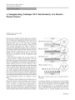
2576 EURASIP Journal on Applied Signal Processing calculated for the full-disk pixel data x j , ( j = 1, N ) as follows: ×104 1.2 0.8 N −1 0.4 1 mean = x = xj, ¯ 0 N 14/ 02/ 02 06/ 03/ 02 26/ 03/ 02 15/ 04/ 02 05/ 05/ 02 j =0 N −1 (a) 1 2 xj − x , variance = ¯ N −1 j =0 1 (1) −1 N −1 xj − x 3 ¯ 1 √ −3 skewness = , 14/ 02/ 02 06/ 03/ 02 26/ 03/ 02 15/ 04/ 02 05/ 05/ 02 N variance j =0 (b) N −1 xj − x 4 ¯ 1 − 3. √ kurtosis = N variance 30 j =0 20 10 The results of the comparison between the Ca II K1 and 0 14/ 02/ 02 06/ 03/ 02 26/ 03/ 02 15/ 04/ 02 05/ 05/ 02 MDI WL data sets for the period February–May 2002 are presented in Figure 3, where (a), (b), and (c) are from the (c) MDI data and (d), (e), and (f) are deduced from the Meudon 4000 data. Figures 3a and 3d present the mean, Figures 3b and 3e present the skewness and Figures 3c and 3f present the kur- 2000 tosis calculated for every daily image. 0 14/ 02/ 02 06/ 03/ 02 26/ 03/ 02 15/ 04/ 02 05/ 05/ 02 The general quality of Meudon images is highly depen- dent on atmospheric conditions at the time of the observa- (d) tion. A number of instrumental artefacts which are diﬃcult to eliminate, such as dust lines, are often present in these im- −4 ages, thus making image unsuitable for automated detection. −8 −12 Together, atmospheric conditions and instrumental artefacts 14/ 02/ 02 06/ 03/ 02 26/ 03/ 02 15/ 04/ 02 05/ 05/ 02 produce the variations shown in Figures 3d, 3e, and 3f. The SOHO satellite data is not subject to clouds as is demon- (e) strated in Figures 3a, 3b, and 3c, though there are dropouts 120 from time to time due to spacecraft problems. Hence, the 80 preprocessing for SOHO images consisted of limb-darkening 40 0 removal only, while for Meudon images it included noise ﬁl- 14/ 02/ 02 06/ 03/ 02 26/ 03/ 02 15/ 04/ 02 05/ 05/ 02 tering with median and/or Gaussian ﬁlters. Hence, the pre- (f) processed images containing quiet Sun pixels with darker and, possibly (for the images in Ca II K1 line) brighter fea- Figure 3: Full-disk data statistics presented for the SOHO/MDI tures superimposed, which are suitable for sunspot detec- continuum (a) mean, (b) skewness, and (c) kurtosis data sets and tion. for the Meudon Observatory Ca II k1 line (d) mean, (e) skewness, For a full-disk solar image free of the limb-darkening, and (f) kurtosis data sets covering February–May 2002. Peaks and the quiet Sun intensity value is established from an image dips in the SOHO/MDI plots correspond to defective data (images) that were automatically rejected by our software (the x-axis refers histogram as the intensity with the highest pixel count (see, to the date of observation and the y -axis to the arbitrary intensity e.g., Figures 4a and 4b). Thus, in a manner similar to [1], by units). analysing the histogram of the ﬂat image, an average quiet Sun intensity, IQSun , can be determined. Basic (binary) morphological operators such as dila- 2.2. Description of the technique tion, closing, and watershed [19, 20] are used in our de- 2.2.1. Automatic detection on the SOHO/MDI tection code. Binary morphological dilation, also known as white-light images Minkowski addition, is deﬁned as The technique developed for the SOHO/MDI data relies on the good quality of the images evident from Figures 3a, A ⊕ B = x : ( B )x ∩ A = ∅ = Ax , (2) 3b, and 3c. This allows a number of parameters, includ- x ∈B ing threshold values as percentages of the quiet Sun inten- where A is the signal or image being operated on and B is sity, to be set constant for the whole data set. Since sunspots are characterised by strong magnetic ﬁeld, the synchronised called the “structuring element.” This equation simply means that B is moved over A and the intersection of B reﬂected and magnetogram data is then used for sunspot veriﬁcation by translated with A is found. Dilation using disk structuring checking the magnetic ﬂux at the identiﬁed feature location.
Automated Recognition of Sunspots 2577 8000 2000 6000 1500 Counts Counts 4000 1000 2000 500 0 0 1.5 × 104 5 × 103 1 × 104 0 200 400 600 800 1000 0 Intensity Intensity (a) (b) Figure 4: Flat image histograms for the (a) Meudon Observatory Ca II K1 line and (b) SOHO/MDI white-light images taken on April 2, 2002 and April 1, 2002, respectively. elements corresponds to isotropic swelling or expansion al- Sun’s rotation around its axis, a SOHO/MDI magnetogram, M , taken at the time TM , is synchronised to the continuum gorithms common to binary image processing. image time TWL via a spatial displacement of the pixels to the Binary morphological erosion, also known as Minkowski position they had at the time TWL in order to obtain the same subtraction, is deﬁned as point of view as those for the continuum. AΘB = x : (B)x ⊆ A = ∅ = Ax . (3) The technique presented in the current paper uses edge x∈B detection with threshold applied on the gradient image. This The equation simply means that erosion of A by B is the set of technique is signiﬁcantly less sensitive to noise than the points x such that B translated by x is contained in A. When global threshold since it uses the background intensity in the the structuring element contains the origin, erosion can be vicinity of a sunspot. We consider sunspots as connected fea- seen as a shrinking of the original image. tures characterised by strong edges, lower than surrounding Morphological closing is deﬁned as dilation followed by quiet Sun intensity, and strong magnetic ﬁeld. Sunspot prop- erosion. Morphological closing is an idempotent operator. erties vary over the solar disk, so a two-stage procedure is Closing an image with a disk structuring element eliminates adopted. First, sunspot candidate regions are deﬁned. Sec- small holes, ﬁlls gaps on the contours, and fuses narrow ond, these are analysed on the basis of their local properties breaks and long, thin gulfs. to determine sunspot umbra and penumbra regions. This is The morphological watershed operator segments images followed by veriﬁcation using magnetic information. A de- into watershed regions and their boundaries. Considering tailed description of the procedure is provided in the pseu- the gray scale image as a surface, each local minimum can docode presented in Algorithm 1. be thought of as the point to which water falling on the sur- Sunspot candidate regions are determined by combining rounding region drains. The boundaries of the watersheds two approaches: edge-detection and low-intensity-region de- lie on the tops of the ridges. This operator labels each water- tection (steps 1–3). First, we obtain a gradient gray-level im- age, ∆ p , from the original preprocessed image, ∆ (Figure 5a) shed region with a unique index, and sets the boundaries to by applying Gaussian smoothing with a sliding window (5 × zero. We apply the watershed operator provided in the IDL library by Research Systemic Inc. to binary image where it 5) followed by Sobel gradient operator (step 1). Then (step 2) ﬂoods enclosed boundaries and thus is used in a ﬁlling algo- we locate strong edges via iterative thresholding of the gradi- ent image starting from initial threshold, T0 , whose value is rithm. For a detailed discussion of mathematical morphol- ogy see the references within the text and numerous books not critical but should be small. The threshold is applied fol- lowed by 5 × 5 median ﬁlter and the number of connected on digital imaging. components Nc and the ratio of the number of edge pixels to The detection code is applied to a “ﬂattened” full-disk SOHO/MDI continuum image, ∆ (Figure 5a), with esti- the total number of disk pixels R are determined. If the ratio mated quiet Sun intensity, IQSun (Figure 4b), image size, solar is too large or the number of components is greater than 250, disk centre pixel coordinates, disk radius, date of observa- the threshold is incremented. The number 250 is based on tion, and resolution (in arcseconds per pixel). Because of the the available recorded maximum number of sunspots which
2578 EURASIP Journal on Applied Signal Processing (a) (b) (c) (d) (e) (f) Figure 5: A sample of the sunspot detection technique applied to the WL disk SOHO/MDI image from April 19, 2002 (presented for a cropped fragment for better resolution): (a) a part of the original image; (b) the detected edges; (c) candidate map; (d) the regions of interest after ﬁltering as masks on original; (e) the detection results before magnetogram veriﬁcation, false identiﬁcation is circled; and (f) the ﬁnal detection results. is around 170.1 Since at this stage of the detection we are deal- into a single candidate region, this limit is increased 250 to ensure that no sunspots are excluded. The presence of noise ing with noise and the possibility of several features joined and ﬁne structures in the original ﬂat image will contribute many low-gradient-value pixels resulting in just a few very 1 The large connected regions, if the threshold is too close to zero. number varies depending on the observer.
Automated Recognition of Sunspots 2579 complete and incomplete sunspot boundaries as well as noise (1) Apply Gaussian smoothing with sliding window 5 × 5 and other features such as the solar limb. followed by the Sobel operator to a copy of ∆. Similarly, the original ﬂat image is iteratively thresholded (2) Using the initial threshold value, T0 , threshold the edge to deﬁne dark regions (step 3). The resulting binary image map and apply the median 5 × 5 ﬁlter to the result. Count the number of connected components, Nc , and contains fragments of sunspot regions and noise. The two the ratio of the number of edge pixels to the total binary images are combined using the logical OR operator number of disk pixels, R (feature candidates, Figures 5b (Figure 5c). The image will contain feature boundaries and and 6b). If Nc is greater than 250 or R is larger than 0.7, blobs corresponding to the areas of high gradient and/or low increase T0 by set value (1 or larger depending on Nc intensity as well as the limb edge. After removing the limb and R) and repeat step 3 from the beginning. boundary, a 7 × 7 morphological closure operator [19, 20] is (3) Similarly, iteratively threshold original ﬂat image to applied to close incomplete boundaries. Closed boundaries deﬁne less than 100 dark regions. Combine (using OR are then ﬁlled by applying a ﬁlling algorithm, based on the operator) two binary images into one binary feature IDL watershed function, [21] to the binary image. A 7 × 7 candidate map (Figure 5c). dilation operator is then applied to deﬁne the regions of in- (4) Remove the edge corresponding to the limb from candidate map and ﬁll the possible gaps in the feature terest which possibly contain sunspots (step 4, Figure 5d, re- outlines using IDL’s morphological closure and gions masked in dark gray). watershed operators (Figures 5d and 6c). In the second stage of detection, these regions are (5) Use blob colouring to deﬁne a region of interest, Fi , as a uniquely labeled using blob colouring algorithm [22] (step set of pixels representing a connected component on the 5) and individually analysed (steps 6-7, Figure 5e). Penum- resulting binary image, B∆ . ¯ bra and umbra boundaries are determined by thresholding (6) Create an empty sunspot candidate map, B∆ , a byte at values Tu and Ts which are functions of the region’s sta- mask which will contain the detection results with pixels tistical properties and quiet Sun intensity deﬁned in step 7. belonging to umbra marked as 2, penumbra as 1. (7) For every Fi extract a cropped image containing Fi and Practically, the formulae for determining Tu and Ts (step 7), deﬁne Ts and Tu : including the quiet Sun intensity coeﬃcients, 0.91, 0.93, 0.6, (i) if |Fi |≤5 pixels, assign the thresholds: for 0.55, are determined by applying the algorithm to a train- penumbra Ts = 0.91IQSun ; for umbra Tu = 0.6IQSun , ing set of about 200 SOHO/MDI WL images. Since smaller (ii) if |Fi | > 5 pixels, assign the thresholds: for regions of interest (step 7(i)) carry less statistical intensity penumbra Ts = max{0.93IQSun ; ( Fi − 0.5∗ ∆Fi )}; information, lower Ts value reduces the probability of false for umbra Tu = max{0.55IQSun ; ( Fi − ∆Fi )}, where identiﬁcation. In order to apply this sunspot detection tech- Fi is a mean intensity and ∆Fi a standard deviation for nique to data sets from other instruments, the values of the Fi . constants appearing in the formulas for Tu and Ts should (8) Threshold a cropped image at this value to deﬁne the candidate umbral and penumbral pixels and insert the be determined for each data set. As mentioned in the in- results back into B∆ (Figures 5e and 6d). Use blob troduction, other authors [6, 7, 8, 9] apply global thresh- colouring to deﬁne a candidate sunspot, Si , as a set of olds at the diﬀerent values of 0.85 or 0.925 for Ts and 0.59 pixels representing a connected component in B∆ . for Tu . (9) To verify the detection results, cross-check B∆ with the In the ﬁnal stage of the algorithm (steps 8-9), we verify synchronised magnetogram, M , as follows: for every the resulting sunspot candidates by determining the maxi- sunspot candidate Si of B∆ extract (i) Bmax (Si ) = max(M ( p) | p ∈ Si ), mum magnetic ﬁeld within the candidate region (Figure 5f). (ii) Bmin (Si ) = min(M ( p) | p ∈ Si ), This information is extracted from synchronised magne- if max(abs(Bmax (Si )), abs(Bmin (Si ))) < 100, then togram M , as described in step 9 when we can verify a disregard Si as noise. sunspot candidate as a sunspot, if this magnetic ﬁeld is higher (10) For each Si extract and store the following parameters: than the magnetic ﬁeld threshold. The latter is chosen to be gravity centre coordinates (Carrington and projective), equal to 100 Gauss, that is appropriate for smallest sunspots, area, diameter, umbra size, number of umbras detected, maximum-minimum-mean photometric intensity (as or pores [18], and is a factor 5 higher than the noise in mag- related to ﬂattened image), maximum-minimum netic ﬁeld measurements by the MDI instrument [15]. magnetic ﬂux, total magnetic ﬂux, and total umbral ﬂux. The method works particularly well for larger features. It also detects a number of smaller features (under 5 pix- Algorithm 1: The pseudocode describing the sunspot detection al- els) for which there is often not enough information in gorithm in SOHO/MDI white-light images. the continuum image to make a decision whether the de- tected feature corresponds to a true feature or an artefact (Figure 5e). This detection is veriﬁed with great accuracy by Imposing an upper limit of 0.7 on the ratio of number of edge using the magnetic ﬁeld information, extracted from the syn- chronised magnetograms (Figure 5f). By comparing Figures pixels to disk pixels excludes this situation. A lower value 5e and 5f we can see that the false detection (marked by a increment in the iterative thresholding loop ensures better circle) between the two top and bottom sunspot groups has accuracy, at the cost of computational time. The increment been remedied. Detected feature parameters are extracted value can also be set as a function of the intermediate values of Nc and R. The resulting binary image (Figure 5b) contains and stored in the ASCII format in the ﬁnal step 10.
2580 EURASIP Journal on Applied Signal Processing (a) (b) (c) (d) (e) Figure 6: Sunspot detection on the Ca II K1 line full-disk image obtained from Meudon Observatory on April 1, 2002: (a) the original image cleaned; (b) the detected edges; (c) the regions found (dilated); (d) the ﬁnal detection results superimposed on original image; and (e) the extract of a single sunspot group from (d). 2.2.2. Technique modiﬁcations for Ca II K1 images The examples of sunspot detection with this technique applied to a Ca II K1 image taken on 2/04/02 are pre- sented in Figure 6. First, the full-disk solar image is pre- The technique described above can also be applied to Ca II processed (Figure 6a) by correcting, if necessary, the shape K1 images with the following modiﬁcations. First, these im- of the disk to a circular one (via automated limb ellipse- ages contain substantial noise and distortions owing to in- ﬁtting) and by removing the limb-darkening as described strumental and atmospheric conditions, so their quality is in Section 2.1.2. Then Sobel edge-detection (similar results much lower than the SOHO/MDI white-light data (see Fig- were also achieved with morphological gradient operation ures 3d, 3e, and 3f). Hence, the threshold in step 7 (i.e., item 7 in the pseudocode) has to be set lower, that is, Ts = [19] deﬁned as the result of subtracting an eroded version max{0.91IQSun ; ( Fi − 0.25∗ ΞFi )} for penumbra and Tu = of the original image from a dilated version of the origi- max{0.55IQSun ; ( Fi − ΞFi )}, for umbra, where ΞFi is the nal image) is applied to the preprocessed image, followed mean absolute deviation of the region of interest Fi . by thresholding in order to detect strong edges (Figure 6b).
Automated Recognition of Sunspots 2581 This over segments the image; and then a 5 × 5 median ﬁl- to be a true feature. In Table 1, case 1, we have included fea- ter and an 8 × 8 morphological closing ﬁlter [19, 20] are tures with sizes over 5 pixels, mean intensities less than the applied to remove noise, to smooth the edges and to ﬁll quiet Sun’s, mean absolute deviations exceeding 20 (which is in small holes in edges. After removing the limb edge, the about 5% of the quiet Sun intensity), principal component ratios less than 2.1. In case 2, we include practically all de- watershed transform [21] is applied to the thresholded bi- nary image in order to ﬁll-in closed sunspot boundaries. tected candidate features by setting the deviation and princi- pal component ratio thresholds to 0.05. Regions of interest are deﬁned, similar to the WL case, The diﬀerences between the manual and automatic via morphological closure and dilation [19, 20]. Candidate sunspot features are then detected by local thresholding us- methods are expressed by calculating the false acceptance rate ing threshold values in the previous paragraph. The can- (FAR) (where we detect a feature and they do not) and the didate features’ statistical properties such as size, principal false rejection rate (FRR) (where they detect a feature and we component coeﬃcients and eigenvalues, intensity mean, and do not). FAR and FRR were calculated for the available ob- servations for the two diﬀerent classiﬁer settings described in mean absolute deviation are then used to aid the removal of false identiﬁcations such as the artefacts and lines, often the previous paragraph. The FAR is lowest for the classiﬁer case 1 and does not exceed 8.8% of the total sunspot number present in the Meudon Observatory images (Figures 6d and 6e). detected on a day. By contrast, FRR is lowest for the classi- ﬁer case 2 and does not exceed 15.2% of the total sunspot It can be seen that on the Ca II K1 image shown in Figure 6 the technique performs as well as on the white-light number. data (Figure 5). However, in many other Ca images the tech- The error rates in Table 1 are the consequences of sev- eral factors related to the image quality. First, diﬀerent seeing nique can still produce a relatively large number of false iden- tiﬁcations for smaller features under 10 pixels where there is conditions can adversely inﬂuence automated recognition re- not enough statistical information to diﬀerentiate between sults; for example, a cloud can obstruct a signiﬁcant portion the noise and sunspots. This raises the problem of veriﬁca- of the disk, thus greatly reducing the quality of that segment of the image, making it diﬃcult to detect the ﬁner details of tion of the detected features that is discussed below. that part of the solar photosphere. Second, some small (less than 5–8 pixels) dust lines and image artefacts can be virtu- 3. VERIFICATION AND ACCURACY ally indistinguishable from smaller sunspots leading to false There are two possible means of veriﬁcation. The ﬁrst option identiﬁcations. assumes the existence of a tested well-established source of Also, in order to interpret the data presented in Table 1, the target data that is used for a straightforward compari- the following points have to be clariﬁed. Sunspot counting methods are diﬀerent for diﬀerent observatories. For exam- son with the automated detection results. In our case, such data would be the records (sunspot drawings) produced by ple, a single large sunspot with one umbra is counted as a a trained observer. However, the number (and geometry) of single feature at Meudon, but can be counted as 3 or more visible/detectable sunspots depend on the time (date) of ob- sunspots (depending on the sunspot group conﬁguration) at the Locarno Observatory. Similarly, there are diﬀerences be- servation (sunspot lifetime can be less than an hour), loca- tion of the observer, wavelength, and resolution (in case of tween the Meudon approach and our approach. For exam- digital imaging). Therefore, this method works best when ple, a large sunspot with several umbras is counted as one the input data for both detection methods is the same. Oth- feature by us, but can be counted as several features by the erwise, a number of diﬀerences can appear naturally when Meudon observer. Furthermore, interpretation of sunspot comparing the two methods. data at Meudon is inﬂuenced by the knowledge of earlier The second option is comparing two diﬀerent data sets de- data and can sometimes be revised in the light of the sub- scribing the same sunspots from images taken on the same sequent observations. Hence, for instance, on April 2, 2002 dates by diﬀerent instruments, and extracting from each data there are 20 sunspots detected at Meudon Observatory. The set a carefully chosen invariant parameter (or set of parame- automated detection applied to the same image yielded 18 ters), such as sunspot area, and looking at its correlation. For sunspots corresponding to 17 of the Meudon sunspots with our technique, both veriﬁcation methods were applied and one of the Meudon sunspots detected as two. Thus, in this the outcome is presented below. case FAR is zero, and FRR is 3. Currently, our automated detection approach is based on 3.1. Veriﬁcation with drawings and synoptic maps extracting all the available information from a single obser- The veriﬁcation of the automated sunspot detection results vation and storing this information digitally. Further analysis started by comparison with the sunspot database produced and classiﬁcation of the archive data is in progress that will al- manually at the Meudon Observatory and published as syn- low us to produce sunspot numbers identical to the existing optic maps in ASCII format. The comparison is shown in spot counting techniques. Table 1. The two cases presented in Table 1 correspond to two For the veriﬁcation of sunspot detection on the ways of accepting/rejecting detected features. In general, by SOHO/MDI images, which have better quality (see Figures considering feature size, shape (i.e., principal components), 3a, 3b, and 3c), less noise, and better time coverage (4 per mean intensity, variance, quiet sun intensity, and proximity day), we used the daily sunspot drawings produced man- to other features, one can decide whether the result is likely ually since 1965 at the Locarno Observatory, Switzerland.
2582 EURASIP Journal on Applied Signal Processing Table 1: The accuracy of sunspot detection and classiﬁcation for Ca II K1 line observations in comparison with the manual set obtained from Meudon Observatory (see the text for description of deﬁned cases 1 and 2). FAR FRR FAR FRR Number of spots Number of spots Number of spots Date (case 1) (case 1) (case 2) (case 2) (Meudon) (case 1) (case 2) 01-Apr-02 16 17 2 1 19 4 1 02-Apr-02 20 18 0 3 18 0 3 03-Apr-02 14 13 0 3 24 10 2 04-Apr-02 13 15 2 2 20 6 1 05-Apr-02 16 18 0 2 18 1 2 06-Apr-02 10 10 0 5 15 5 5 07-Apr-02 11 9 1 5 13 4 4 08-Apr-02 14 17 3 2 22 7 0 09-Apr-02 16 17 0 2 17 0 2 10-Apr-02 12 12 0 4 14 1 3 11-Apr-02 12 9 0 7 10 1 7 12-Apr-02 18 20 2 0 21 3 0 14-Apr-02 20 23 2 2 34 13 2 15-Apr-02 13 16 1 4 18 2 3 16-Apr-02 10 13 3 1 19 9 1 17-Apr-02 11 11 1 1 13 2 0 18-Apr-02 12 11 1 1 12 1 0 19-Apr-02 11 14 0 0 15 1 0 20-Apr-02 13 10 0 2 11 1 2 21-Apr-02 9 8 1 1 15 7 0 22-Apr-02 12 13 1 0 15 3 0 23-Apr-02 14 13 0 1 15 1 0 24-Apr-02 18 15 0 3 17 0 1 25-Apr-02 17 13 0 3 17 2 1 27-Apr-02 9 7 0 1 9 2 1 28-Apr-02 9 10 1 0 11 2 0 29-Apr-02 8 12 5 0 20 13 0 The Locarno manual drawings are produced in accordance presented in Figure 7b with those available as ASCII ﬁles ob- with the technique developed by Waldmeier [23] and the tained from the drawings of about 365 daily images obtained results are stored in the solar index data catalogue (SIDC) in 2003 at the US Air Force/NOAA (taken from National at the Royal Belgian Observatory, Brussels [24]. While the Observatory for Astronomy and Astrophysics National Geo- physical Data Centre, US [25]), revealed a correlation coeﬃ- Locarno observations are subject to seeing conditions, this is counterbalanced by the higher resolution of live obser- cient of 96% (Figure 7a). This is a very high accuracy of de- vations (about 1 arcsecond). We have compared the re- tection that ensures a good quality of extracted parameters sults of our automated detection in white-light images with within the resolution limits deﬁned by a particular instru- the available drawings in Locarno for June–July 2002, as ment. well as for January–February 2004 along with a number Further veriﬁcation of sunspot detection in WL images of random dates in 2002 and 2003 (about 100 daily draw- can be obtained by comparing sunspot area statistics with so- ings with up to 100 sunspots per drawing). The compari- lar activity index such as sunspot numbers. Sunspot numbers son has shown a good agreement (∼ 95%–98%). The auto- are generated manually from sunspot drawings [24] and are mated method detects all sunspots visually observable in the related to the number of sunspot groups. The ﬁrst attempt SOHO/MDI WL observations. The discrepancies are found to compare the sunspot area statistics detected by us with the at the level of sunspot pores (smaller structures), and can sunspot numbers revealed a correlation of up to 86% (see be explained by the time diﬀerence between the observa- Zharkov and Zharkova [26]). For accurate comparison clas- tions and by the lower resolution of the SOHO/MDI im- siﬁcation of sunspots into groups is required. Manually this ages. is done using sunspot magnetic ﬁeld polarity tags and the property that neighbouring sunspots with opposite magnetic 3.2. Veriﬁcation with the NOAA data set ﬁeld polarities are paired into groups. Implementation of the automated classiﬁcation of sunspots into groups is the scope Comparison of temporal variations of the daily sunspot ar- of a future paper. eas extracted from the EGSO solar feature catalogue in 2003
Automated Recognition of Sunspots 2583 A number of physical and geometrical parameters of millionth of solar hemishphere ×104 sunspot features are extracted and stored in the rela- Total sunspot areas in 2 tional database along with run-length encoded umbra and 1.5 penumbra regions within the bounding rectangle for each sunspot. The database is accessible via web services and 1 (http://solar.inf.brad.ac.uk) website. 0.5 In order to signiﬁcantly reduce the errors contained in 0 acceptance and rejection rate coeﬃcients FARs and FRRs and 09/ 02/ 03 10/ 04/ 03 09/ 06/ 03 08/ 08/ 03 07/ 10/ 03 06/ 12/ 03 validate the detection with the existing activity index [25], Date of observation the sunspot candidate classiﬁcation into groups has to be im- (a) plemented. This can be done by examining the adjacent ob- servations, their magnetic polarity, and values, and that is, Total sunspot areas in 120 the scope of a forthcoming paper. 100 sq. degrees 80 ACKNOWLEDGMENT 60 40 The research has been done for European Grid of Solar Ob- 20 servations (EGSO) funded by the European Commission 0 09/ 02/ 03 10/ 04/ 03 09/ 06/ 03 08/ 08/ 03 07/ 10/ 03 06/ 12/ 03 within the IST ﬁfth framework, Grant IST-2001-32409. Date of observation REFERENCES (b) [1] M. Steinegger, M. Vazquez, J. A. Bonet, and P. N. Brandt, “On Figure 7: A comparison of temporal variations of daily sunspot ar- the energy balance of solar active regions,” Astrophysical Jour- eas extracted in 2003 from the (a) USAF/NOAA archive, US, and nal, vol. 461, pp. 478–498, April 1996. from the (b) solar feature catalogue with the presented technique. [2] D. V. Hoyt and K. H. Schatten, “Group sunspot numbers: a new solar activity reconstruction,” Solar Physics, vol. 179, no. 1, pp. 189–219, 1998. [3] D. V. Hoyt and K. H. Schatten, “Group sunspot numbers: 4. THE CONCLUSIONS a new solar activity reconstruction,” Solar Physics, vol. 181, no. 2, pp. 491–512, 1998. New improved techniques are presented for automated [4] M. Temmer, A. Veronig, and A. Hanslmeier, “Hemispheric sunspot detection on full-disk solar images obtained in the sunspot numbers Rn and Rs : Catalogue and N-S asymmetry Ca II K1 line from the Meudon Observatory (∼ 300 im- analysis,” Astronomy & Astrophysics, vol. 390, pp. 707–715, ages) and in WL from the MDI instrument aboard the SOHO August 2002. [5] G. A. Chapman and G. Groisman, “A digital analysis of satellite (10 082 images). sunspot areas,” Solar Physics, vol. 91, pp. 45–50, March 1984. The technique applies automated image cleaning pro- [6] G. A. Chapman, A. M. Cookson, and J. J. Dobias, “Observa- cedures for elimination of limb-darkening and noncircular tions of changes in the bolometric contrast of sunspots,” As- image shape. Edge-detection methods and global threshold- trophysical Journal, vol. 432, no. 1, pp. 403–408, 1994. ing methods are used to produce initial image segmentation. [7] G. A. Chapman, A. M. Cookson, and D. V. Hoyt, “Solar ir- The resulting oversegmentation is remedied using a median radiance from Nimbus-7 compared with ground-based pho- tometry,” Solar Physics, vol. 149, no. 2, pp. 249–255, 1994. ﬁlter followed by morphological closing operations to close [8] M. Steinegger, P. N. Brandt, J. M. Pap, and W. Schmidt, boundaries. A watershed region ﬁlling operation, 7 × 7 mor- “Sunspot photometry and the total solar irradiance deﬁcit phological closing and dilation operators are used to deﬁne measured in 1980 by ACRIM,” Astrophysics and Space Science, the regions of interest possibly containing sunspots. Each re- vol. 170, no. 1-2, pp. 127–133, 1990. gion is then examined separately and the values of thresh- [9] P. N. Brandt, W. Schmidt, and M. Steinegger, “On the umbra- olds used to deﬁne sunspot umbra and penumbra bound- penumbra area ratio of sunspots,” Solar Physics, vol. 129, pp. 191–194, September 1990. aries are determined as a function of the full-disk quiet Sun [10] T. Pettauer and P. N. Brandt, “On novel methods to deter- intensity value and statistical properties of the region (such as mine areas of sunspots from photoheliograms,” Solar Physics, mean intensity, standard, deviation, and absolute mean de- vol. 175, no. 1, pp. 197–203, 1997. viation). The sunspots detected in WL are veriﬁed using the ´ [11] M. Steinegger, J. A. Bonet, and M. Vazquez, “Simulation SOHO/MDI magnetogram data. of seeing inﬂuences on the photometric determination of The detection results for the selected months in 2002– sunspot areas,” Solar Physics, vol. 171, no. 2, pp. 303–330, 1997. 2003 show a good agreement with the Meudon manual syn- [12] D. G. Preminger, S. R. Walton, and G. A. Chapman, “Solar optic maps and a very good agreement with the Locarno feature identiﬁcation using contrasts and contiguity,” Solar manual drawings (95%–98%). The temporal variations of Physics, vol. 202, no. 1, pp. 53–62, 2001. sunspot areas detected in 2003 with the presented technique [13] M. Turmon, J. M. Pap, and S. Mukhtar, “Statistical pattern from white-light images revealed a very high correlation recognition for labeling solar active regions: application to (96%) with those produced manually at the National Obser- SOHO/MDI imagery,” Astrophysical Journal, vol. 568, no. 1, vatory for Astronomy and Astrophysics (NOAA), US. part 1, pp. 396–407, 2002.
2584 EURASIP Journal on Applied Signal Processing S. Ipson graduated in 1969 with a First Class ¨ [14] L. Gyori, “Automation of area measurement of sunspots,” So- with Honors degree in applied physics from lar Physics, vol. 180, no. 1-2, pp. 109–130, 1998. [15] P. H. Sherrer, R. S. Bogart, R. I. Bush, et al., “The solar oscilla- the University of Bradford, following peri- tions investigation-Michelson Doppler imager,” Solar Physics, ods spent at the Rutherford Appleton Lab- vol. 162, no. 1/2, pp. 129–188, 1995. oratory, BP Research Laboratory, Sunbury, [16] V. V. Zharkova, S. S. Ipson, S. I. Zharkov, A. Benkhalil, J. and the AEA, Winfrith. After carrying out Aboudarham, and R. D. Bentley, “A full-disk image standard- theoretical and experimental work at AERE, isation of the synoptic solar observations at the Meudon Ob- Harwell, and the Universities of Bradford, servatory,” Solar Physics, vol. 214, no. 1, pp. 89–105, 2003. Oxford, and Heidelberg, he was awarded a [17] J. Canny, “A computational approach to edge detection,” IEEE Ph.D. degree in theoretical nuclear physics Trans. Pattern Anal. Machine Intell., vol. 8, no. 6, pp. 679–698, in 1975 from the University of Bradford. He is currently a Senior 1986. Lecturer in the Department of Cybernetics, University of Bradford [18] C. W. Allen, Astrophysical Quantities, Athlone Press, London, and his present research interests are digital image restoration, pat- UK, 1973. tern recognition, and 3D reconstruction from multiple images. [19] J. Serra, Image Analysis and Mathematical Morphology, vol. 1, Academic Press, London, UK, 1988. A. Benkhalil received a B.Eng. degree in [20] G. Matheron, Random Sets and Integral Geometry, John Wiley computer engineering from The Higher In- & Sons, New York, NY, USA, 1975. stitute of Electronics, Libya, in 1988, an [21] P. T. Jackway, “Gradient watersheds in morphological scale- M.S. degree in real-time electronic systems space,” IEEE Trans. Image Processing, vol. 5, no. 6, pp. 913–921, from University of Bradford, UK, in 1996, 1996. and a Ph.D. degree from the same univer- [22] A. Rosenfeld and J. L. Pfaltz, “Sequential operations in digital sity in 2001 on a project entitled “An FPGA- picture processing,” Journal of the Association for Computing based real-time autonomous video surveil- Machinery, vol. 13, no. 4, pp. 471–494, 1966. lance system.” He is currently a full-time [23] M. Waldmeier, The Sunspot Activity in the Years 1610–1960, postdoctoral Research Assistant for the Eu- Sunspot Tables, Schulthess Publisher, Zurich, Switzerland, 1961. ropean Grid of Solar Observations (EGSO), University of Bradford. [24] Solar Index Data Catalogue, Belgian Royal Observatory, His current research interests include image processing, computer http://sidc.oma.be/products/. vision, and real-time systems design. [25] NOAA National Geophysical Data Center, http://www.ngdc. noaa.gov/stp/SOLAR/ftpsunspotregions.html. [26] S. I. Zharkov and V. V. Zharkova, “Statistical properties of sunspots and their magnetic ﬁeld detected from full disk SOHO/MDI images in 1996–2003,” Adv. Space Res., in press. S. Zharkov obtained his B.A. (Hons) de- gree in mathematics from Cambridge Uni- versity in 1996, his Ph.D. degree from Glas- gow University in 2000. He is a postdoctoral Research Assistant at Bradford University, a key developer of the solar feature catalogues for the European Grid of Solar Observa- tions (EGSO) Project. His present interests include digital image processing, solar dy- namo theory, and diﬀerential geometry. V. Zharkova obtained an M.S. degree (ﬁrst class with distinction) in applied mathe- matics from Kiev State University in 1975, a Ph.D. degree in astrophysics from the Main Astronomical Observatory, National Academy of Sciences of Ukraine in 1984, Advanced Certiﬁcate in computing sciences from Kiev State University in 1989. She worked in the Physics and Applied Math- ematics Department, Kiev State University, and in the Physics and Astronomy Department, Glasgow Univer- sity, UK. Currently she is a Professor in applied mathematics at the Department of Cybernetics, Bradford University, UK, and leads the Solar Imaging Research Group. Her current research interests are solar feature recognition from solar images obtained from various space and ground-based observations,ﬂare-induced wave recogni- tion, energy release and transport in solar ﬂares, and prediction of solar activity.

CÓ THỂ BẠN MUỐN DOWNLOAD

TL.01: Bộ Tiểu Luận Triết Học

207 tài liệu

1446 lượt tải

ERROR:connection to 10.20.1.98:9315 failed (errno=111, msg=Connection refused)
ERROR:connection to 10.20.1.98:9315 failed (errno=111, msg=Connection refused)

THÔNG TIN

TRỢ GIÚP

HỖ TRỢ KHÁCH HÀNG

Theo dõi chúng tôi

Chịu trách nhiệm nội dung:

Nguyễn Công Hà - Giám đốc Công ty TNHH TÀI LIỆU TRỰC TUYẾN VI NA

LIÊN HỆ

Địa chỉ: P402, 54A Nơ Trang Long, Phường 14, Q.Bình Thạnh, TP.HCM

Hotline: 093 303 0098

Email: support@tailieu.vn