http://www.iaeme.com/IJMET/index.asp 718 editor@iaeme.com
International Journal of Mechanical Engineering and Technology (IJMET)
Volume 10, Issue 03, March 2019, pp. 718-725. Article ID: IJMET_10_03_075
Available online at http://www.iaeme.com/ijmet/issues.asp?JType=IJMET&VType=10&IType=3
ISSN Print: 0976-6340 and ISSN Online: 0976-6359
© IAEME Publication Scopus Indexed
TOURISM PROMOTION, TOURISM REVENUES
AND SECTORAL OUTPUTS IN THAILAND
Bundit Chaivichayachat
Department of Economics, Faculty of Economics, Kasetsart University
Bangkok, Thailand
ABSTRACT
Since 2010, tourism promoting policies have been implemented to drive economic
growth and also economic development in Thailand. Government allocated a
significant budget to promote tourism sector. As a result, tourism revenues have also
been increased significantly. The increasing in the number of visitors induced the
domestic final demand and the output in tourism related sectors. However, the
different group of visitors will response to the tourism promoting policy in the
different ways. Following the Johansen system cointegration, the results indicate that
the tourism revenue in each group of visitors was response to the difference set of
macroeconomic factors. The estimated normalized cointegration vectors confirm the
positive relationship between government budget for promoting tourism and tourism
revenue for all groups of visitors. For the sectoral analysis, tourism revenue,
naturally, induces final demand and initiates output only in a few sectors. According
to the results, the policies are (1) continuously promote tourism sectors in term of
government budget, (2) set up a specific policy for each group of visitors and (3)
income re-distribution to the sector which are not related to tourism sector.
Key words: Thai Tourism, Input-Output Table, Bridge Matrix, Tourism Revenue
Cite this Article: Bundit Chaivichayachat, Tourism Promotion, Tourism Revenues
and Sectoral Outputs in Thailand, International Journal of Mechanical Engineering
and Technology, 10(3), 2019, pp. 718-725.
http://www.iaeme.com/IJMET/issues.asp?JType=IJMET&VType=10&IType=3
1. INTRODUCTION
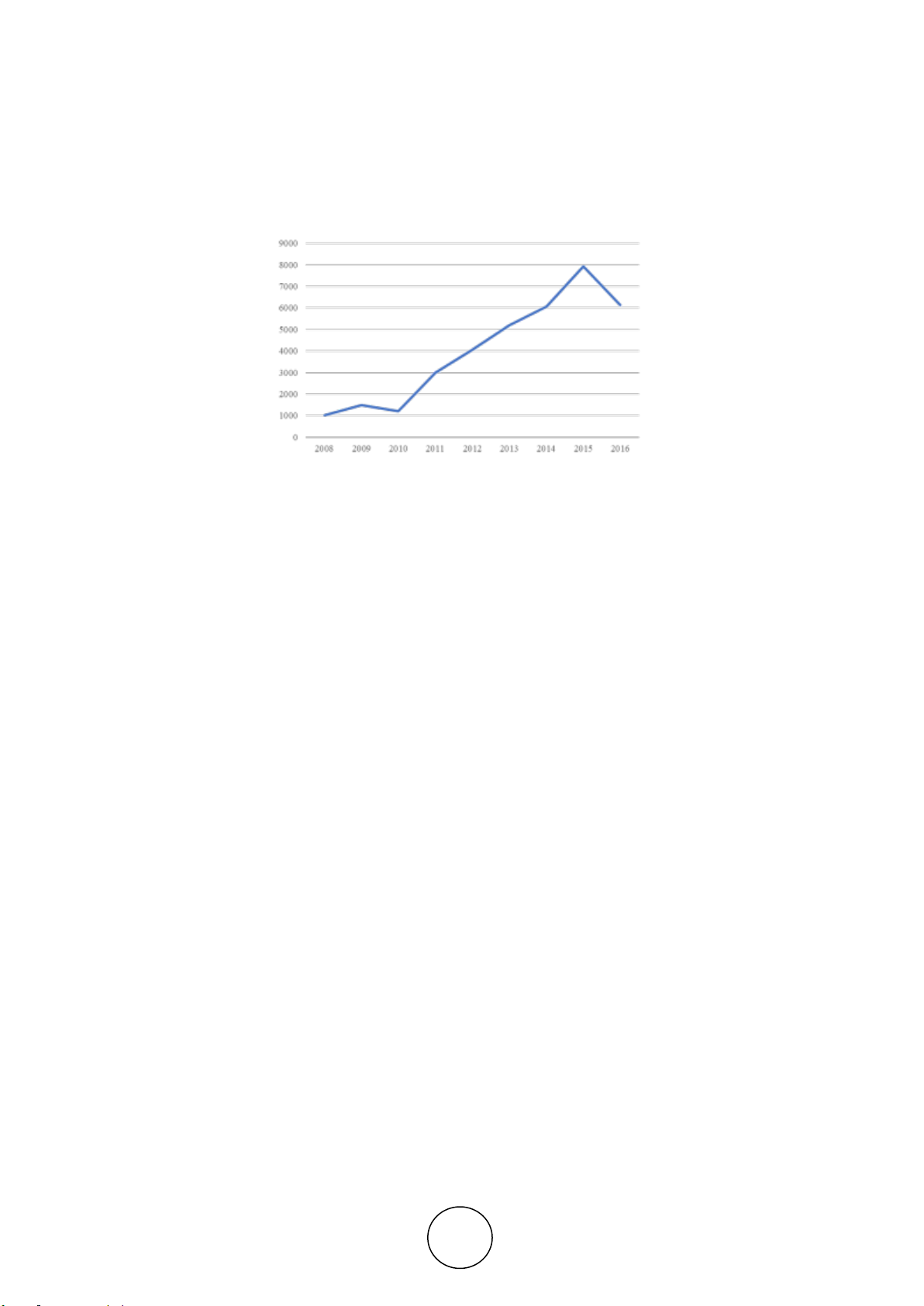
Since 2010, tourism promoting policies have been implemented to drive economic growth
and economic development in Thailand. Government allocated a significant budget to
promote tourism sector. (Figure 1) The target is to induce the number of tourists and
excursionists to spend and to stay more in Thailand. Not only the foreign visitors but also for
the Thai’s visitors. As a result, the number of 4 groups of visitors have been increased
significantly both in term of number and in term of revenue. The increasing in visitors
induced the domestic final demand for the output in tourism related sectors. However, we
cannot find the research which aimed to explore the results of the tourism promoting policy in