9
EM Eigenfrequencies in a
Spheroidal Cavity
9.1
INTRODUCTION
Computation of eigenfrequencies in EM cavities is useful in various applica-
t ions. However, analytical calculation of these eigenfrequencies is severely
limited by the boundary shape of these cavities. In this chapter, the interior
boundary value problem in a prolate spheroidal cavity with a perfectly con-
ducting wall and axial symmetry is solved analytically. By applying Maxwell’s
equations to the boundary, it is possible to obtain an analytical expression of
the eigenfrequency fnSo using spheroidal wave functions regardless of whether
the parameter c is small or large.
An inspection of the plot of a series of fnSa values (confirmed in [64])
indicates that variation of fnSo with the coordinate parameter < is of the form
fn&) = fnS(0)[ 1 + g(l)@ + gt2)/c4 + gc3)/t6 + 9
l
l
] when c is small. By
fitting the fnSo, 5 evaluated onto an equation of its derived form, the first four
expansion coefficients - g(O), g(l), gc2) and g13) are determined numerically
using the least squares method. The method used to obtain these coefficients
is direct and simple, although the assumption of axial symmetry may restrict
its applications to those eigenfrequencies f72Sml, where m’ = 0.
245
Spheroidal Wave Functions in Electromagnetic Theory
Le-Wei Li, Xiao-Kang Kang, Mook-Seng Leong
Copyright 2002 John Wiley & Sons, Inc.
ISBNs: 0-471-03170-4 (Hardback); 0-471-22157-0 (Electronic)

246
EM EIGENFREQUENCIES IN A SPHEROIDAL CAVITY
9.2
THEORY AND FORMULATION
9.2.1
Background Theory
The prolate spheroidal body under consideration is shown in Fig. 9.1. In view
of the fact that Mathematics handles only vector differential operations in the
prolate spheroidal coordinates in accordance with the notations used in the
book by Moon and Spencer [9, pp. 28-291, a temporary change of coordinates
is necessarv. The new notation used is shown in Fig. 2.1.
a
Fig. 9.1 Geometry of the spheroidal cavity.
As noted by Moon and Spencer (91, the vector Helmholtz equation is more
complicated than the scalar counterpart, and its solution using the variable-
separation principle may sometimes cause new problems. This is especially
true in rotational systems like that of the spherical coordinates or spheroidal
coordinates. In spheroidal coordinates, the solving of vector boundary value
problems is further complicated by the fact that the vector wave equation
is not exactly separable in spheroidal coordinates. Although another more
general analysis has been performed using the vector wave functions, formed
by operating on the scalar spheroidal wave functions with vector operators,
the validity of the results obtained is doubtful. In view of these limitations,

THEORY AND FORMULATION
247
several assumptions are made in the formulation of the current boundary
problem in order to provide a truer, more accurate picture.
9.2.2 Derivation
With axial symmetry assumed, it is possible to separate the field components
into Et, Eq, and I$ for the TM mode and Ht, &, and E4 for the TE mode.
First, the TM mode is considered. With axial symmetry, I74 can be as-
sumed simply as
Hc#l = F(c, W(c, 7). (9 1)
.
By applying the Maxwell equations
dB
VxE = ---, (9.2a)
dD
VxH = dt, (9.2b)
and using the formulation of V x X in the spheroidal coordinates where
vxx =
Q77 = d2K2 - v2)
4(1 - 72) ’
iI< = d2(C2 - v2)
4K
2-l) ’
94 = %(1 - v2>(C2 - l),
(9 3)
.
(9.4a)
(9.4b)
(9.4c)
the following equations can be obtained:
a2;p (C2
_ 1) +
,py
- 1
(c2 + amn) - c2tf2 + A] F(c,C) = 0,
a2g9q1
_ r72) _ ,py
- (c2 + amn) - c2q2 + i-t-;;?] G(c, Q-) = 0.
(9.5a)
(9.5b)

248
EM NGENFREQUENCIES IN A SPHEROIDAL CAVITY
In the case when the semimajor axis of the spheroidal surface is close to
the semiminor axis (d = dm << l), the parameter c2 (c = kd/2) used
in the summation with anzn will diminish due to the decreasing value of d2.
Thus Eqs. (9.5a) and (9.5b) will be reduced to
-
[
Qrmn - c2y2 + $-+
1
G(c,C) = 0.
(9.6a)
(9.6b)
Comparison of Eqs. (9,.5a) and (9.5b) with Eqs. (2.8a) and (2.8b) indicates
that the solutions to the differential equations are in fact given by
J”(c, <) = BnRil,) (C, C>,
G(c 7) - C
‘) - s(l)(c 7)
n In 7
(9.7a)
(9.7b)
(i.e., the radial and angular functions with m = 1). In the equations above,
Bn
and Cn are unknowns to be determined from the EM boundary condi-
tions. Hence, the magnetic field component for the TM modes can in fact be
expressed as
H4 = BnCnRln (C, 5)Sln (C7 V) Y (9 8)
.
and the electric field is therefore expressed as
Es = A
jwq/iq
J&&G 5)
X
BnCndw
[
~Sln(G rl) d
37
+ +&7 7) 7
1
(9.9a)
E rl =
(9.9b)
A 2
-
- d(C
2 - l)(l - $) l
To obtain the resonance condition, & must be zero at the surface 5 = 50
of the perfectly conducting spheroidal cavity. From Eq. (9.9b), this requires
that
’ [Rln(CJf)j/~] 1
at
= 0.
(9.10)
t=t0
Thus, by finding the roots of the equation above, the eigenfrequency of the
TM mode can be found.

NUMERICAL RESULTS FOR TE MODES
249
By principle of duality, the fields components for the TE mode can be
obtained by substituting & for H4, -& for Et, and -JY? for E?, , respectively.
Hence, the resonance condition for the TE modes can be obtained by setting
E+ = 0 at 5 = 50. From Eq. (9.8), the boundary condition requires that
&n(c, <>I(=&) = 0.
(9.11)
9.3 NUMERICAL RESULTS FOR TE MODES
9.3.1 Numerical Calculation
Using the package created in previous chapters, the zeros of the radial func-
tion, as required by the resonance condition in Eq. (9.11) can be found in a
straightforward way. This is because coding the radial function into a package
(1)
offers convenience of treating &,&, {) as if it is normal function like cosine
and sine. Hence, the command FindRoot in Mathematics can be employed
to solve directly for the zeros of &&,<). This is achieved by means of the
Newton-Raphson method in the software program.
In our program, the iterations will stop when the next iterative value com-
puted is less than lo? As in any Newton’s method implementation, an
initial guess is required. The spherical Bessel function zeros of various orders
are assigned as the first guess. This will provide faster convergence since in
the case considered, the spheroidal coordinates can actually be approximated
roughly by the spherical coordinates. And from Stratton [7], the resonance
condition is given by j, (/w) = 0 in the spherical coordinates. Under the
circumstance considered, 4 (in spheroidal coordinates) + kr (in spherical
coordinated), thus the required values of g must be in the region around
zeros of the spherical Bessel functions.
It is observed from practical calculations that in the region when @ is large,
FindRoot using Newton’s method is capable of evaluating the zeros accurately
at a very high speed. However, at the same time, it is also observed that the
rate will decrease drastically in the region where @ is small. This can be
explained by the proximity of the initial guess. A series of zeros, spanning the
range from t = 100 to < = 1000, were collected at irregular intervals.
From the work done by Kokkorakis and Roumeliotis [65], it can be shown,
after some manipulations, that the series of values of g that satisfies Rln(c, 5) =
0, are, in fact, governed by an equation of the form
c(C)5 = 90
[l+~(~)+~($)2+~($)3+**j, (9.12)
where go,gl,g2, l . . are unknown coefficients to be determined.