
Quy ho ch và x lý s li u th c nghi mạ ử ố ệ ự ệ
GV: PGS.TS.Nguy n Doãn Ýễ
Ti u lu n môn h cể ậ ọ
Quy ho ch và x lý s li u th c nghi mạ ử ố ệ ự ệ
Làm t bài 3.27 đ n bài 3.38ừ ế
H c Viên: Vũ Quang L ngọ ươ 1 L p:CNCK810ớ

Quy ho ch và x lý s li u th c nghi mạ ử ố ệ ự ệ
GV: PGS.TS.Nguy n Doãn Ýễ
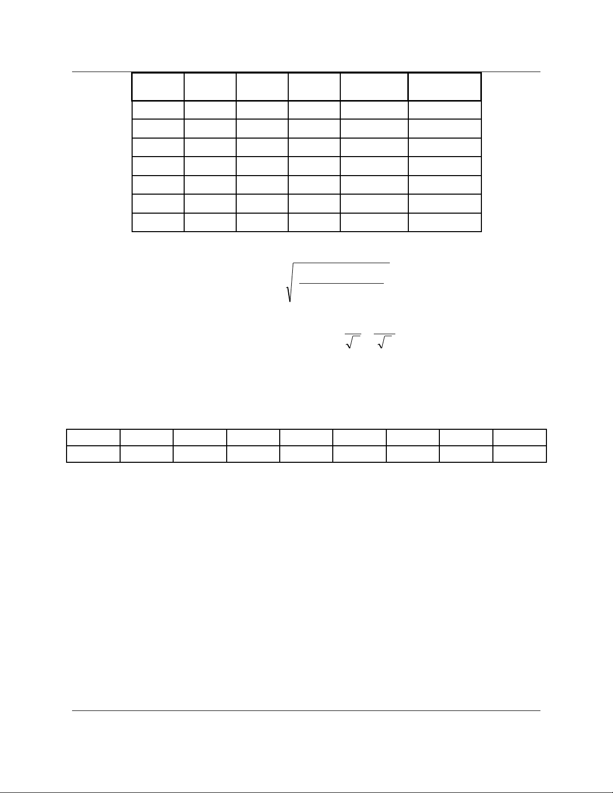
3.27. The following data are expected to follow a linear relation of the form
y = ax + b. Obtain the best linear relation in accordance with a least-squares
analysis. Calculate the standard deviation of the data from the predicted straight-
line relation.
x 0.9 2.3 3.3 4.5 5.7 6.7
y 1.1 1.6 2.6 3.2 4.0 5.0
Solution:
Các d li u sau đây đ c d ki n s th c hi n theo m t quan h tuy nữ ệ ượ ự ế ẽ ự ệ ộ ệ ế
tính y = ax + y. Có đ c m i quan h tuy n tính theo phượ ố ệ ế ân tích bình ph ngươ
nh nh tỏ ấ . Tính toán đ l ch chu n c a d li u t các d đoán quan h đ ngộ ệ ẩ ủ ữ ệ ừ ự ệ ườ
th ng.ẳ
T ph ng trình có d ng: y = ax + bừ ươ ạ
STT x y xy x2
10.9 1.1 0.99 0.81
2 2.3 1.6 3.68 5.29
3 3.3 2.6 8.58 10.89
4 4.5 3.2 14.4 20.25
5 5.7 4 22.8 32.49
6 6.7 5 33.5 44.89
T nổ
g23.4 17.5 83.95 114.6
We calculate the value of a and b:
67,0
4,236,114.6
5.17.4,2395,83.6
)(
)().(
222 =
−
−
=
−
−
=∑ ∑
∑ ∑∑
ii
iiii
xxn
yxyxn
a
30,0
4,236,114.6
4,23.95,836,114.5,17
)(
)().())((
222
2
=
−
−
=
−
−
=∑ ∑
∑ ∑∑∑
ii
iiiii
xxn
xyxxy
b
Thus, the desired relation is: y = 0,67x + 0,30
H c Viên: Vũ Quang L ngọ ươ 2 L p:CNCK810ớ
Quy ho ch và x lý s li u th c nghi mạ ử ố ệ ự ệ
GV: PGS.TS.Nguy n Doãn Ýễ
x y xy x2(yi-axi-b)2
1 0.9 1.1 0.99 0.81 0.04
2 2.3 1.6 3.68 5.29 0.06
3 3.3 2.6 8.58 10.89 0.01
4 4.5 3.2 14.40 20.25 0.01
5 5.7 4 22.80 32.49 0.02
6 6.7 5 33.50 44.89 0.04
Sum 23.40 17.50 83.95 114.62 0.18
21,0
2
)(
)error( Standard
2
=
−
−−
=∑
n
baxy ii
σ
086,0
6
21,0
)(Deviation Standard === n
m
σ
σ
3.28. The following data points are expected to follow a funtional variation
of y = axb. Obtain the values of a and b from graphical analysis.
x 1.21 1.35 2.40 2.75 4.50 5.1 7.1 8.1
y 1.20 1.82 5.00 8.80 19.50 32.5 55.0 80.0
Solution:
y = axb(a>0, x>0)
Suy ra: lgy = lga + blgx
Đ t:ặ Y = lgy; A = lga; X = lgx
Ta có hàm tuy n tính m i:ế ớ
Y = A + bX
Tính toán t ng t bài 3.27 ta có: A = 0,097; b = 1,003ươ ự
T đó tính đ c a = 1,251ừ ượ
H c Viên: Vũ Quang L ngọ ươ 3 L p:CNCK810ớ
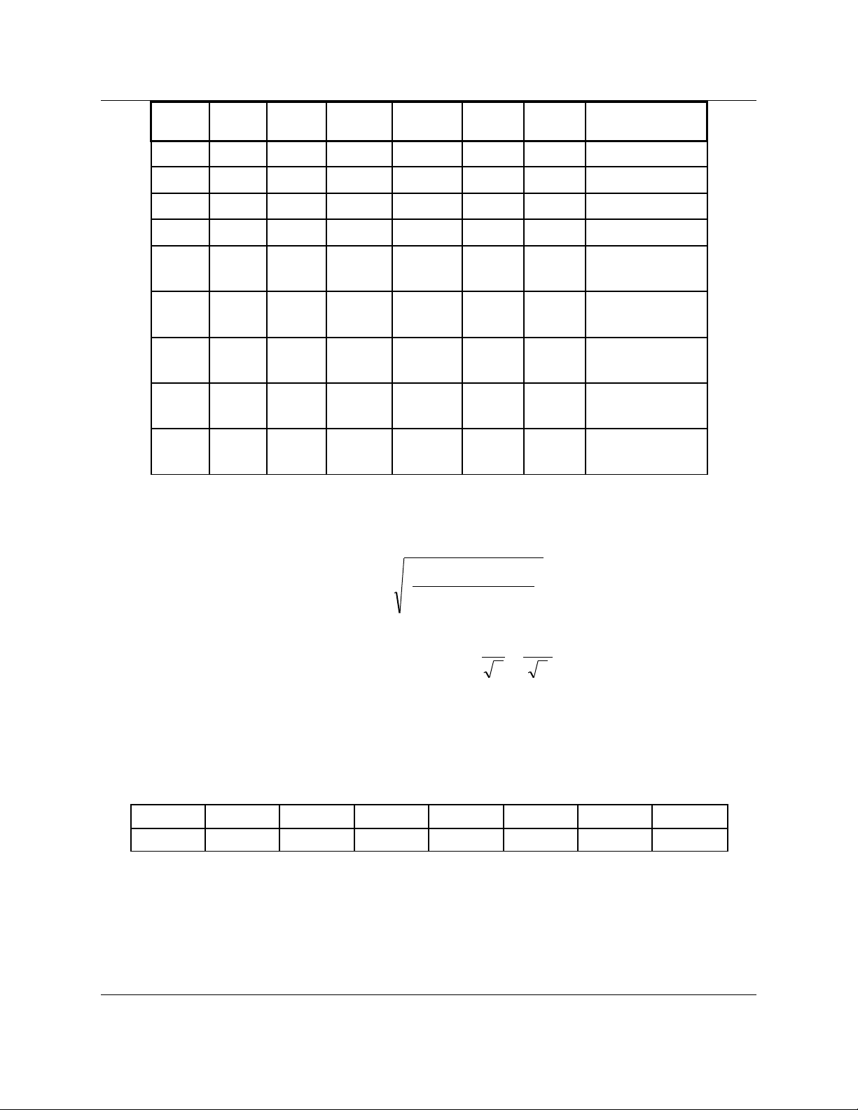
Quy ho ch và x lý s li u th c nghi mạ ử ố ệ ự ệ
GV: PGS.TS.Nguy n Doãn Ýễ
STT x y X=lgx Y=lgy XY X2(Yi-AXi-b)2
11.21 1.20 0.083 0.079 0.007 0.007 0.87
21.35 1.82 0.130 0.260 0.034 0.017 0.57
32.40 5.00 0.380 0.699 0.266 0.145 0.12
42.75 8.80 0.439 0.944 0.415 0.193 0.01
54.50
19.5
0
0.653 1.290 0.843 0.427 0.05
65.10
32.5
0
0.708 1.512 1.07 0.501 0.19
77.10
55.0
0
0.851 1.740 1.481 0.725 0.43
88.10
80.0
0
0.908 1.903 1.729 0.825 0.66
T nổ
g 4.153 8.428 5.844 17.25 2.90
695,0
2
)(
)error( Standard
2
=
−
−−
=∑
n
baxy ii
σ
246,0
6
21,0
)(Deviation Standard === n
m
σ
σ
3.29. The following data points are expected to follow a funtional
variation of y = aebx. Obtain the values of a and b from graphical analysis.
x 0 0,43 1,25 1,40 2,60 2,90 4,30
y 9,4 7,1 5,35 4,2 2,6 1,95 1,15
Solution:
y = aebx
Suy ra lny = lna + bx
H c Viên: Vũ Quang L ngọ ươ 4 L p:CNCK810ớ
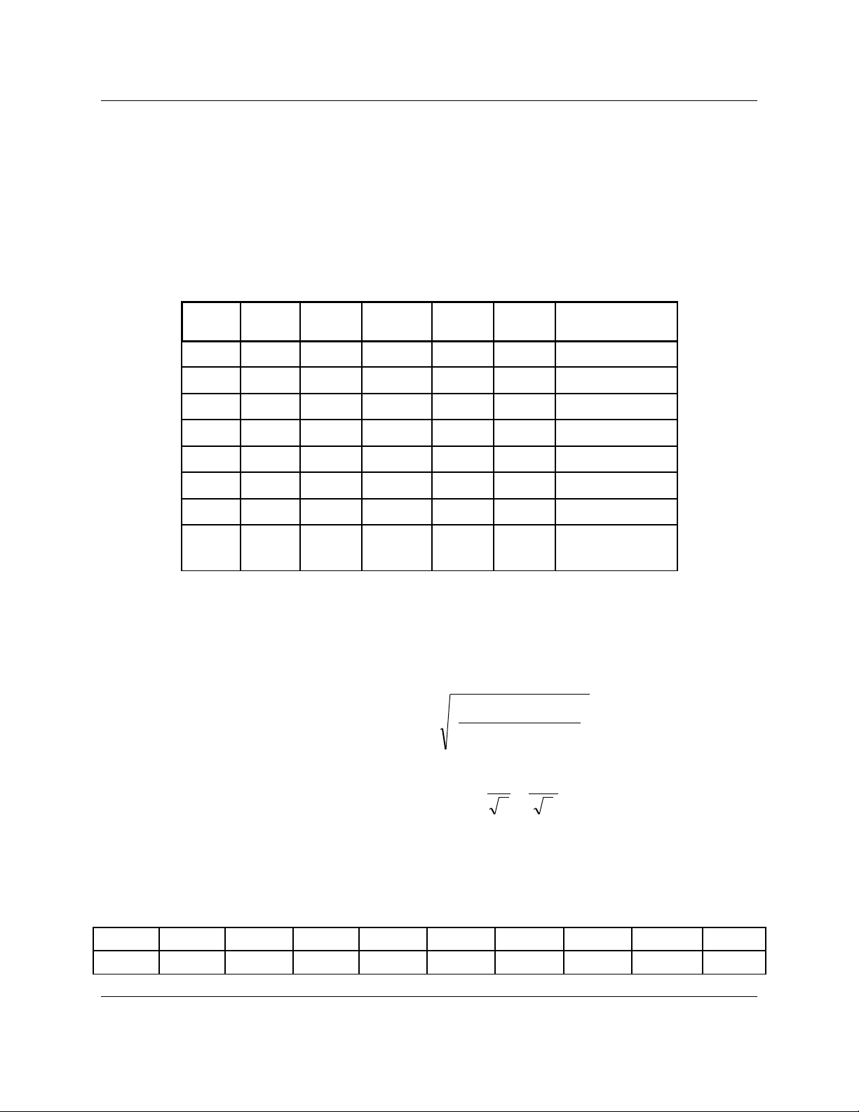
Quy ho ch và x lý s li u th c nghi mạ ử ố ệ ự ệ
GV: PGS.TS.Nguy n Doãn Ýễ
Đ t: Y = lny;ặA = lna
Ta có hàm tuy n tính m i: ế ớ Y = A + bx
T ng t ta có: A = -0,492;ươ ự b = 2,203
Suy ra: a = eA= 0,611
V y hàm tuy n tính ban đ u có d ng: ậ ế ầ ạ y = 0,611e2,203x
STT y x Y=lny xY x2(Yi-Axi-b)2
19.40 0.00 2.241 0 0 0.0015
27.10 0.43 1.960 0.843 0.185 0.0009
35.35 1.25 1.677 2.096 1.563 0.0081
44.20 1.40 1.435 2.009 1.96 0.0061
52.60 2.60 0.956 2.484 6.76 0.0011
61.95 2.90 0.668 1.937 8.41 0.0114
71.15 4.30 0.140 0.601 18.49 0.0030
T nổ
g
31.7
512.88 9.076 9.97 37.37 0.0321
08,0
2
)(
)error( Standard
2
=
−
−−
=∑
n
baxy ii
σ
03,0
6
21,0
)(Deviation Standard === n
m
σ
σ
3.30. The following heat-transfer data point are expected to follow a
funtional form of N = aRb. Obtain the values of a and b from graphical analysis and
also by the method of least square:
R 12 20 30 40 100 300 400 1000 3000
N 2 2,5 3 3,3 5,3 10 11 17 30
H c Viên: Vũ Quang L ngọ ươ 5 L p:CNCK810ớ


![Bộ 2 đề thi cuối kì 2 Xác suất thống kê năm 2015 có đáp án [kèm đáp án chi tiết]](https://cdn.tailieu.vn/images/document/thumbnail/2025/20250815/nganga_07/135x160/19511755252739.jpg)

![Bộ 12 đề thi học kì 2 môn Xác suất & Thống kê có đáp án [kèm lời giải chi tiết]](https://cdn.tailieu.vn/images/document/thumbnail/2025/20250815/nganga_07/135x160/75281755252733.jpg)